IB Mathematics: Analysis and Approaches
Calculus Formulae for AA SL & AA HL
A complete guide to the shared Calculus content: limits, derivatives, tangents, integration, graph behaviour, optimization, kinematics, definite integrals and areas.
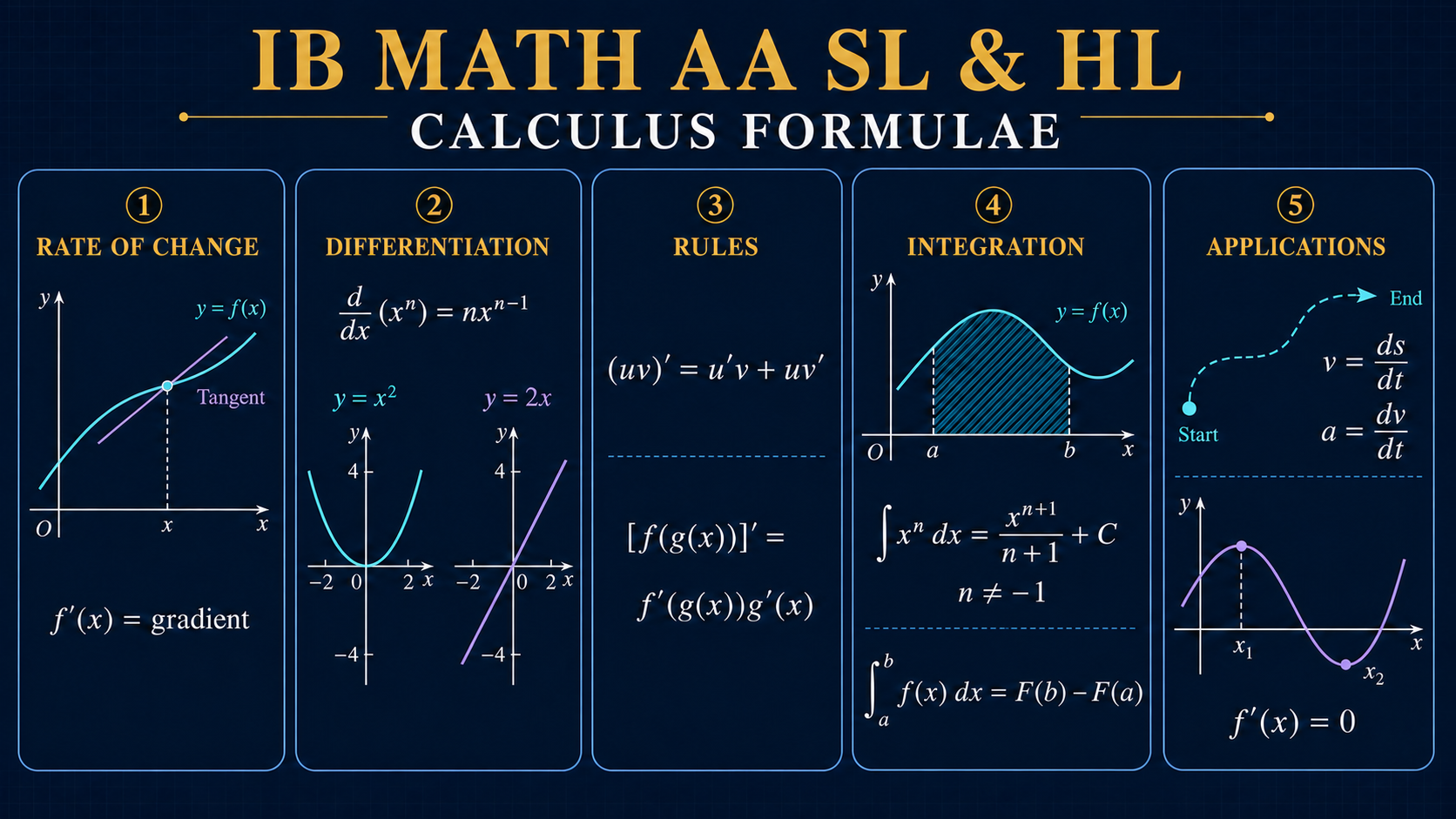
What Calculus content is shared by AA SL and AA HL?
Calculus studies change and accumulation. Differentiation describes instantaneous rate of change and local graph behaviour; integration reverses differentiation and measures accumulated change. In Mathematics AA, these ideas connect directly to functions, modelling, optimization, motion and area. HL students require all SL techniques before adding the AHL extension, so the shared material must be mastered rather than treated as preliminary revision.
| Current section | Main idea | Required skill |
|---|---|---|
| SL 5.1 | Informal limit; derivative as gradient and rate | Estimate a limit and interpret derivative notation |
| SL 5.2 | Increasing and decreasing functions | Connect the sign of f′ to graph behaviour |
| SL 5.3 | Power rule for integer powers | Differentiate polynomial expressions |
| SL 5.4 | Tangents and normals | Find a gradient and construct a line equation |
| SL 5.5 | Initial integration, boundary conditions and area with technology | Find an antiderivative and determine its constant |
| SL 5.6 | Standard derivatives, chain, product and quotient rules | Differentiate composite and combined functions |
| SL 5.7 | Second derivative and related graphs | Connect f, f′ and f″ |
| SL 5.8 | Extrema, optimization, concavity and inflexion | Classify stationary points and solve optimization problems |
| SL 5.9 | Kinematics | Relate displacement, velocity, acceleration and distance |
| SL 5.10 | Extended antiderivatives and reverse chain rule | Integrate standard and recognizable composite forms |
| SL 5.11 | Definite integrals analytically | Use an antiderivative to evaluate accumulation |
| SL 5.12 | Areas using integration | Set up positive geometric area between boundaries |
The course expects both analytical reasoning and technology. You should know when an exact derivative or antiderivative is available, when a GDC is appropriate, and how to communicate the setup. A numerical value without a correct derivative, integral or interpretation may not answer the question.
Limits and the meaning of a derivative
A limit describes the value a function approaches as its input approaches a point. At SL, limits are introduced informally through tables and graphs rather than formal symbolic techniques. The distinction between an approached value and an actual value matters: a graph can approach a height even when the point is missing or the function is defined differently at that input.
The derivative f′(x) is the gradient function. At a particular input x=a, f′(a) is the gradient of the tangent to y=f(x) at that point. In a context, it is an instantaneous rate: if s(t) is displacement, then s′(t) is velocity. Derivative notation should carry the relevant variables:
Average rate of change across an interval is a secant gradient:
Instantaneous rate describes one moment and is obtained from the derivative. Do not substitute a tiny interval and call the result exact unless the question asks for an approximation.
Worked example: interpret a derivative
A tank’s volume is V(t)=500+40t−2t² litres. Then dV/dt=40−4t litres per minute. At t=6, the rate is 16 L/min, meaning the volume is increasing at that instant. The derivative becomes zero at t=10; after that, the model predicts decreasing volume.
Increasing and decreasing intervals
- If f′(x)>0 on an interval, f is increasing there.
- If f′(x)<0 on an interval, f is decreasing there.
- If f′(x)=0 at a point, the tangent is horizontal, but the point is not automatically a maximum or minimum.
A sign chart for f′ is often clearer than a sentence. Find every relevant zero or undefined point of the derivative, divide the domain into intervals, test a value in each interval and translate the signs into graph behaviour.
Core differentiation formulae
The power rule is the foundation for polynomial differentiation. Differentiate each term and preserve constant multipliers.
For SL 5.3 the exponents are integers; SL 5.6 extends the power rule to rational exponents. Constants differentiate to zero. Rewrite roots and reciprocals as powers when that makes the rule clearer: √x=x1/2 and 1/x²=x−2.
Worked example: polynomial and rational powers
For f(x)=3x5−4x−2+7√x−9, write the root as x1/2. Then f′(x)=15x4+8x−3+(7/2)x−1/2. The original function and derivative require x>0 because of both the square root and negative powers.
Standard derivatives
| f(x) | f′(x) | Domain reminder |
|---|---|---|
| xn | nxn−1 | Respect the original power’s real domain |
| sin x | cos x | Angles in radians for calculus |
| cos x | −sin x | Remember the negative sign |
| ex | ex | All real x |
| ln x | 1/x | x>0 |
Tangents and normals
At x=a, the tangent gradient is mt=f′(a). The tangent passes through (a,f(a)), so point-gradient form gives:
A normal is perpendicular to the tangent. When f′(a) is non-zero and finite, its gradient is mn=−1/f′(a). Handle horizontal and vertical cases separately: a horizontal tangent has a vertical normal.
Worked example: tangent and normal
For f(x)=x³−2x at x=2, f(2)=4 and f′(x)=3x²−2, so f′(2)=10. The tangent is y−4=10(x−2). The normal gradient is −1/10, giving y−4=−(1/10)(x−2).
In a context, interpret the gradient with units. If a cost function is measured in dollars and input is items, its derivative has units dollars per item and may be interpreted as marginal cost near that production level.
Integration as anti-differentiation
An antiderivative of f is a function whose derivative is f. Indefinite integration represents the whole family of antiderivatives, so it includes an arbitrary constant C. The constant disappears under differentiation, which is why it cannot be recovered from the derivative alone.
A boundary or initial condition determines C. Integrate first, substitute the known point, solve for the constant and then present the complete function.
Worked example: boundary condition
Given dy/dx=3x²+x and y=10 when x=1, integrate to obtain y=x³+(1/2)x²+C. Substitution gives 10=1+1/2+C, so C=17/2. Therefore y=x³+(1/2)x²+17/2.
A definite integral is a number rather than a family, so it does not include C. It measures signed accumulation. Area above the x-axis contributes positively and area below contributes negatively. Geometric area is never negative, so a curve that crosses the axis requires the interval to be split.
Chain, product and quotient rules
SL 5.6 includes the rules needed to differentiate composite, multiplied and divided functions. Before choosing a rule, identify the outer structure. Algebraic simplification may turn a complicated-looking expression into an easier sum of powers.
Chain rule
Differentiate the outside while keeping the inside, then multiply by the derivative of the inside.
Chain-rule example
For y=ex²+2, the outside derivative remains exponential and the inside derivative is 2x. Thus dy/dx=2x ex²+2. For y=sin(3x−1), the derivative is 3cos(3x−1).
Product rule
Product-rule example
If f(x)=x²ex, take u=x² and v=ex. Then f′(x)=2x ex+x²ex=x ex(x+2). Factoring helps when solving f′(x)=0.
Quotient rule
Quotient-rule example
For g(x)=ln x/x, u=ln x and v=x. Then g′(x)=[(1/x)x−ln x]/x²=(1−ln x)/x², with x>0.
Second derivative and graph behaviour
The second derivative is the derivative of the derivative. If f describes position, f′ describes velocity and f″ describes acceleration. Graphically, f″ tracks how the gradient changes.
- f″(x)>0: the graph is concave up and its gradient is increasing.
- f″(x)<0: the graph is concave down and its gradient is decreasing.
- A possible point of inflexion occurs where concavity may change; f″=0 alone is not sufficient.
Relationships among the graphs are powerful. Zeros of f′ correspond to stationary points of f. Local maxima and minima of f′ can correspond to zeros of f″. Where f′ lies above its axis, f increases; where it lies below, f decreases.
Worked example: derivative sign table
Let f′(x)=(x−1)(x−4). It is positive for x<1, negative for 1<x<4 and positive for x>4. Therefore f increases, then decreases, then increases. The point at x=1 is a local maximum and the point at x=4 is a local minimum.
Stationary points, optimization and inflexion
A stationary point satisfies f′(x)=0. Classify it using a sign change of the first derivative or the second derivative test:
- f′ changes + to −: local maximum.
- f′ changes − to +: local minimum.
- If f″(a)>0 at a stationary point: local minimum.
- If f″(a)<0 at a stationary point: local maximum.
- If f″(a)=0: the test is inconclusive.
A point of inflexion is where concavity changes. It may have zero or non-zero gradient. Check the sign of f″ on both sides rather than declaring every solution of f″=0 an inflexion. For example, y=x4 has f″(0)=0 but does not change concavity at the origin.
Optimization workflow
- Define variables and constraints. Include units and the feasible domain.
- Create one objective function. Express the quantity to maximize or minimize in one variable.
- Differentiate. Find critical points from f′=0 or undefined derivative.
- Check candidates. Classify stationary points and compare endpoints when the domain is closed.
- Interpret. Answer in the original variables with appropriate units and accuracy.
Worked example: maximize a rectangle
A rectangle has perimeter 40 cm. If one side is x, the other is 20−x, with 0<x<20. Area A(x)=x(20−x)=20x−x². Then A′=20−2x, so x=10. Because A″=−2<0, this is a maximum. The rectangle is a 10 cm square with maximum area 100 cm².
Kinematics: displacement, velocity and acceleration
Velocity is signed; speed is |v|. Positive velocity means displacement increases, while negative velocity means it decreases. Acceleration describes change in velocity, not necessarily speeding up. An object speeds up when velocity and acceleration have the same sign and slows down when their signs differ.
Displacement over an interval is the signed integral of velocity. Total distance requires the integral of speed, so split at every time when velocity changes sign:
Worked example: distance versus displacement
Let v(t)=3t²−12t+9 for 0≤t≤4. Factor to 3(t−1)(t−3), so velocity changes sign at 1 and 3. For displacement, integrate over [0,4] directly. For distance, evaluate the signed integral separately on [0,1], [1,3] and [3,4], then add the absolute values. Ignoring the sign changes would give net displacement, not total travel.
If acceleration and one velocity value are known, integrate acceleration and use the velocity condition to determine the constant. Integrate again and use a displacement condition if the position function is required. Each integration introduces its own constant.
Extended integration formulae
| Integrand | Antiderivative | Condition |
|---|---|---|
| xn | xn+1/(n+1)+C | n≠−1 |
| 1/x | ln|x|+C | x≠0 on an interval |
| ex | ex+C | All real x |
| sin x | −cos x+C | Radians |
| cos x | sin x+C | Radians |
For a linear inner function, compensate for its derivative. For example:
Reverse chain rule, integration by inspection or substitution recognizes a derivative of the inside multiplied by a function of the inside:
Worked example: reverse chain rule
Evaluate ∫2x(x²+1)4 dx. Let u=x²+1, so du=2x dx. The integral becomes ∫u4du=u5/5+C. Hence the answer is (x²+1)5/5+C. Differentiate to verify both the power and inner factor.
Worked example: logarithmic pattern
For ∫sin x/cos x dx, let u=cos x, so du=−sin x dx. The integral is −∫(1/u)du=−ln|u|+C=−ln|cos x|+C.
Definite integrals and geometric area
If F′=f, then the fundamental relationship is:
A definite integral gives signed area relative to the x-axis. For geometric area between y=f(x) and the x-axis, find every crossing and integrate the absolute contribution. For area between upper curve u(x) and lower curve l(x):
First solve the intersection equations to obtain correct boundaries. The “upper” curve may change, so sketch or test intervals. Reversing the order produces a negative integral, which signals that the geometric setup is wrong.
Worked example: area between two curves
Find the enclosed area between y=2x and y=x². Intersections satisfy x²=2x, giving x=0 and 2. On (0,2), 2x lies above x². Therefore area=∫02(2x−x²)dx=[x²−x³/3]02=4−8/3=4/3 square units.
Technology may evaluate integrals that lack an accessible analytical antiderivative, but you should still write the correct integral with bounds. The setup shows which quantity is accumulated and is often the central mathematical step.
Connecting algebra, graphs and calculus
A derivative is itself a function. Factoring f′ reveals stationary points and sign intervals; solving f″=0 identifies candidates for concavity change; integrating a rate reconstructs accumulated quantity. Algebraic forms matter: a factored derivative supports sign analysis, while an expanded derivative may be easier to obtain.
For f(x)=x³−3x²−9x+2, the derivative is 3x²−6x−9=3(x−3)(x+1). The factorization immediately gives stationary inputs −1 and 3. The second derivative is 6x−6, so f″(−1)<0 identifies a local maximum and f″(3)>0 identifies a local minimum. The second derivative changes sign at x=1, giving the inflexion input.
Exact results before decimals
Keep exact fractions, radicals, logarithms and multiples of π until a decimal is required. Exact stationary inputs often reveal symmetry or permit exact coordinates. Rounding a boundary before evaluating an area can accumulate error. When a GDC is required, retain guard digits and round once in the final line.
Domain and endpoint awareness
Calculus does not erase domain restrictions. The derivative of ln x applies only for x>0; a rational derivative excludes denominator zeros; a square-root derivative may fail at an endpoint even when the original function is defined there. In optimization on a closed interval, compare interior critical points with both endpoints. The greatest or least value may occur at a boundary rather than a stationary point.
Technology and GDC workflow
- Write the mathematics first. State the derivative, equation or definite integral the calculator will evaluate.
- Check mode and syntax. Use radians for calculus with trigonometric functions; enter brackets and bounds carefully.
- Choose a justified window. Predict critical points, zeros and domain restrictions.
- Use the correct operation. Derivative-at-point, zero, minimum, maximum and numeric integral solve different tasks.
- Verify the output. Compare with sign, units, bounds and graph shape.
- Report properly. Give the requested accuracy and contextual conclusion.
Technology is particularly useful for exploring the relationship among f, f′ and f″, solving derivative equations without simple exact roots and evaluating definite integrals numerically. A graph should confirm reasoning, not replace the domain, equation or interval.
AA SL and HL Calculus exam workflow
- Identify the requested quantity. Gradient, rate, coordinate, maximum, displacement, distance and area are different outputs.
- Record domain and units. These control valid candidates and interpretation.
- Choose the correct rule. Simplify first, then select power, chain, product or quotient.
- Show the setup. Write f′=0, the tangent equation or a definite integral before evaluating.
- Classify and compare. A stationary point needs a sign or second-derivative test; optimization may need endpoints.
- Split sign-changing quantities. Distance and geometric area require positive contributions.
- Preserve accuracy. Keep exact values or guard digits until the final line.
- Interpret. Finish with variables, units and the meaning in context.
Common mistakes and how to repair them
| Mistake | Why it fails | Repair |
|---|---|---|
| Using average gradient for an instantaneous rate | A secant and tangent answer different questions | Differentiate and evaluate at the specified input |
| Forgetting the inner derivative | The chain rule is incomplete | Mark outside and inside before differentiating |
| Differentiating a product term-by-term | (uv)′ is not u′v′ | Use u′v+uv′ |
| Missing +C | An indefinite integral is a family | Add the constant before applying a boundary condition |
| Adding +C to a definite integral | The constants cancel in F(b)−F(a) | Evaluate the bounds directly |
| Calling every f′=0 point an extremum | A stationary inflexion is possible | Use first- or second-derivative evidence |
| Using f″=0 alone for inflexion | Concavity might not change | Test the sign of f″ on both sides |
| Confusing distance and displacement | Negative velocity cancels in displacement | Split at velocity zeros and add absolute contributions |
| Integrating lower minus upper | Geometric area becomes negative | Sketch and use upper minus lower |
| Ignoring endpoints in optimization | An absolute optimum may occur at a boundary | Compare every feasible candidate |
Mixed worked problems
Problem 1: stationary points and classification
For f(x)=x³−6x²+9x+2, f′=3x²−12x+9=3(x−1)(x−3). Stationary inputs are 1 and 3. Since f″=6x−12, f″(1)=−6 gives a local maximum and f″(3)=6 gives a local minimum. Their coordinates are (1,6) and (3,2).
Problem 2: tangent parallel to a line
Find points on y=x³−3x where the tangent is parallel to y=9x+4. Parallel gradients are equal, so 3x²−3=9. Thus x²=4 and x=±2. The points are (2,2) and (−2,−2).
Problem 3: recover a function from its derivative
Given f′(x)=6x−4 and f(2)=7, integrate: f(x)=3x²−4x+C. Substitution gives 7=12−8+C, so C=3. Therefore f(x)=3x²−4x+3.
Problem 4: area crossing the x-axis
Find the geometric area between y=x²−1 and the x-axis from −2 to 2. The curve crosses at −1 and 1. It is positive on [−2,−1] and [1,2] but negative on [−1,1]. Therefore area=∫−2−1(x²−1)dx−∫−11(x²−1)dx+∫12(x²−1)dx. Symmetry can simplify the calculation, but the sign split must remain conceptually clear.
Problem 5: velocity model
A particle has v(t)=t²−6t+8. It is at rest when (t−2)(t−4)=0, so t=2 or 4. Acceleration is a(t)=2t−6. The velocity is positive before 2, negative between 2 and 4, and positive after 4; a distance calculation across these times must split at both zeros.
A practical 14-day Calculus revision plan
| Days | Focus | Evidence of mastery |
|---|---|---|
| 1 | Limits, gradient and rate interpretation | Explain average versus instantaneous change |
| 2-3 | Power rule and standard derivatives | Differentiate mixed functions with correct domains |
| 4 | Tangents and normals | Construct both line equations with units where relevant |
| 5-6 | Chain, product and quotient rules | Select and combine rules without prompts |
| 7 | Second derivative and graph relationships | Build sign charts and classify points |
| 8 | Optimization and inflexion | Check constraints, candidates and endpoints |
| 9 | Kinematics | Distinguish velocity, speed, displacement and distance |
| 10-11 | Indefinite integration and reverse chain rule | Integrate standard forms and use conditions |
| 12 | Definite integrals and area | Choose bounds and split sign-changing regions |
| 13 | Mixed GDC and non-GDC questions | Show valid setups and controlled rounding |
| 14 | Error review | Redo every missed question and state the repair rule |
How to build reliable Calculus solutions
Knowing a formula is only the starting point. Strong AA Calculus work follows a chain of decisions: identify the quantity that changes, choose a function and domain, decide whether the question asks for a rate or an accumulation, apply the appropriate rule, and interpret the result in context. This habit matters because two questions can contain almost identical algebra while asking for different mathematical objects. A derivative gives a local rate, gradient or sensitivity. An integral gives accumulated change, signed area or a recovered function. Before writing any symbols, finish the sentence “I need the derivative because…” or “I need the integral because…”. That ten-second check prevents many method errors.
Translate the command term before calculating
Words such as increasing, decreasing, stationary, maximum rate, minimum value, total distance and area enclosed point to different procedures. “Find when the population is increasing” means solve an inequality involving the first derivative. “Find the greatest population” means find feasible stationary points and compare them with relevant endpoints. “Find the total change” means integrate the rate, while “find the total amount” may also require adding an initial value. In motion, “when the particle changes direction” requires a zero of velocity with a sign change; merely solving v=0 identifies candidates. Translate the language into a one-line mathematical target before manipulating the function.
Control the domain from the beginning
A correct algebraic answer can still be invalid for the model. A length cannot be negative, time may be restricted to a stated interval, a logarithm requires a positive argument, and a denominator cannot be zero. Write the domain beside the model, not after the calculation. When optimization produces two stationary inputs, reject a value only with a stated reason such as “outside 0≤t≤12” or “would give a negative radius.” For an absolute maximum or minimum on a closed interval, evaluate the function at every stationary point inside the interval and at both endpoints. A derivative test classifies local behaviour; it does not automatically compare every feasible value.
Choose differentiation rules from the function’s structure
Read a function from the outside inward. A power of a bracket, a trigonometric function of another expression, an exponential with a nontrivial exponent, or a logarithm of a function signals the chain rule. Two variable expressions multiplied together signal the product rule. One variable expression divided by another may call for the quotient rule, although an algebraic rewrite can sometimes make the power and product rules faster. For example, (x²+1)/x can be rewritten as x+x−1 before differentiation. The best method is the one that is valid, transparent and least likely to generate avoidable algebra.
Rule-selection example
Differentiate y=x²sin(3x). The outer structure is a product, so keep both factors and apply the product rule. The derivative of sin(3x) also requires the chain rule. Therefore dy/dx=2xsin(3x)+3x²cos(3x). A useful check is to ask whether each original factor appears in one term of the product-rule result. Omitting the inner derivative 3 is a separate chain-rule error, so both structures must be checked.
Use derivative signs as evidence, not decoration
A sign chart should communicate an argument. Mark critical inputs in order, test the sign of f′ in each interval, and then state the behaviour of f. A positive-to-negative change proves a local maximum; negative-to-positive proves a local minimum. If there is no sign change, the stationary point is not a local extremum. For concavity, repeat the logic with f″. A change from positive to negative means the graph changes from concave up to concave down; the reverse means concave down to concave up. This sign-change evidence is more reliable than memorizing a graph shape and is essential when a second-derivative value equals zero.
Make integration answers carry meaning
An antiderivative is incomplete without +C unless bounds are present or a boundary condition immediately determines the constant. A definite integral has a numerical value but that value may be signed. If a velocity graph lies below the time-axis, its integral contributes negative displacement; distance requires the absolute contribution. If a curve crosses the x-axis, geometric area requires splitting at every intercept and reversing negative pieces. If two curves enclose a region, identify which is upper on each interval. A quick sketch and one test value are often enough. Always finish with suitable units: square units for geometric area, length units for displacement and distance, and context-specific units for accumulated quantities.
Accumulation example
Suppose water enters a tank at rate r(t) litres per minute and the tank contains 120 litres at t=0. The integral ∫08r(t)dt is the net amount added during eight minutes, not automatically the final volume. The final volume is 120+∫08r(t)dt. If r can be negative, the integral still gives net change because outflow subtracts. If the question instead asks for the total quantity of water that moved through a pipe, the interpretation may require integrating the magnitude of the rate.
Show calculator work in an examinable form
A graphing calculator can locate intersections, zeros, extrema and definite integrals, but the written solution must reveal the mathematics being solved. State an equation such as f′(x)=0, give the interval used, record the relevant numerical solution, and then interpret it. Do not write only “from GDC.” When graphing, choose a window that contains the stated domain and inspect whether additional solutions lie outside the first view. Keep unrounded values in the calculator and round only the final answer to the requested accuracy. If a later calculation uses an earlier result, store the full value instead of retyping a rounded display.
Check an answer with an independent idea
Every Calculus result has a quick consistency test. Differentiate an antiderivative to recover the integrand. Check that a tangent gradient equals the derivative at its contact point. Confirm that a normal gradient is the negative reciprocal when the tangent is neither horizontal nor vertical. Substitute a stationary input into the original function to get its coordinate. Inspect the sign of a rate before and after a claimed turning time. Estimate a definite integral from the graph so an impossible sign or magnitude stands out. Dimensional reasoning is especially powerful: differentiating distance with respect to time should produce distance per time, while integrating velocity with respect to time should return distance units.
Turn errors into a reusable revision record
After practice, label each mistake by cause rather than copying the correct answer. Useful labels include wrong target, wrong rule, missing inner derivative, algebra error, domain ignored, endpoint missed, signed area confused with geometric area, premature rounding and weak interpretation. Beside each label, write a short repair instruction. For example: “Before quotient rule, check whether division by a power of x can be rewritten”; “For distance, solve v=0 and split”; or “For an absolute optimum, compare endpoints.” Reattempt the same question without notes, then solve a different question requiring the same decision. This converts one corrected exercise into a method that transfers to unfamiliar exam problems.
Common questions
Is this guide for both AA SL and AA HL?
Yes. It covers current SL 5.1-5.12, studied by both levels. HL students also need the AHL material beginning at 5.13.
Are product and quotient rules required at AA SL?
Yes. They appear within current SL 5.6 alongside the chain rule and standard derivatives.
Is differentiation from first principles shared SL content?
The shared course introduces the derivative informally through gradient and limits. Formal first-principles and more advanced limit work belong to the AHL extension; use the HL-only guide for that boundary.
When do I use the chain rule?
Use it when one differentiable function is inside another, such as sin(3x−1), ex² or (x²+1)5.
Why is there a constant C in an indefinite integral?
All functions that differ by a constant have the same derivative. A boundary condition is needed to select one member of the family.
How do I tell a maximum from a minimum?
Use the sign change of the first derivative or the sign of the second derivative at a stationary point. If the second derivative is zero, use another test.
Does f double-prime equal zero prove an inflexion?
No. The second derivative must change sign, meaning the graph changes concavity. The zero is only a candidate.
What is the difference between displacement and distance?
Displacement is signed net change and equals the integral of velocity. Distance is total travel and equals the integral of speed, so negative-velocity sections contribute positively.
Can a calculator evaluate the integral for me?
Technology can evaluate many definite integrals, but you should still write the correct integrand and bounds and interpret whether the result is signed accumulation or area.
Should I use degrees or radians in Calculus?
Use radians for standard trigonometric derivative and integral formulae unless a problem explicitly establishes another context.
What Calculus topics are AA HL-only?
The AHL extension includes advanced limits, implicit differentiation and related rates, additional derivatives and integrals, more advanced integration techniques, volumes, differential equations and series-related work. Follow the dedicated HL guide for the exact current sequence.
Will the course change for examinations from May 2029?
The updated AA course begins teaching in August 2027 and first assessment is May 2029. The IB describes limited reductions with no new content. Use your school’s guide for your assessment session.
Continue your IB Math AA revision
- Calculus formulae for AA HL only
- Functions formulae for AA SL and HL
- Number and algebra formulae for AA SL and HL
- Geometry and trigonometry formulae for AA SL and HL
- Statistics and probability formulae for AA SL and HL
Official references: IB Mathematics: Analysis and Approaches guide; IB Diploma Programme mathematics overview; IB Mathematics AA curriculum update.
RevisionTown is an independent educational resource and is not affiliated with or endorsed by the International Baccalaureate Organization. Always use the subject guide and instructions supplied for your examination session.