IB Mathematics: Analysis and Approaches Higher Level
IB Math AA HL Calculus Formulae
A complete educator-written guide to the higher-level calculus extension: first principles, l’Hôpital’s rule, implicit differentiation, related rates, advanced integration, volumes of revolution, differential equations, Euler’s method and Maclaurin series.

What is included in AA HL calculus?
Higher-level calculus is not a separate subject placed after the standard-level course. It extends the same central ideas—change, accumulation, approximation and modelling—using more powerful analytical methods. A student must still differentiate ordinary functions, apply the chain, product and quotient rules, classify stationary points, integrate standard forms, calculate area and interpret motion. The AHL material then adds formal reasoning, difficult limits, implicit relationships, broader function families, stronger integration techniques, volumes, first-order differential equations and infinite series.
The current official guide organizes the extension as AHL 5.12 to AHL 5.19. The numbering is useful for checking coverage, but successful revision should be organized by connections. Partial fractions from number and algebra feed into integration and differential equations. Inverse functions from the functions topic explain inverse-trigonometric derivatives. Graph transformations clarify Maclaurin substitutions. Vectors and trigonometry can supply the geometric context for rates of change.
| AHL section | Main content | What a student should be able to do |
|---|---|---|
| AHL 5.12 | Continuity, differentiability, limits, first-principles derivatives and higher derivatives | Explain local behaviour, derive a polynomial derivative from its definition and use higher-order notation |
| AHL 5.13 | Indeterminate limits | Recognize zero-over-zero or infinity-over-infinity and use l’Hôpital’s rule or a series appropriately |
| AHL 5.14 | Implicit differentiation, related rates and optimisation | Differentiate linked variables and test all feasible candidates, including endpoints |
| AHL 5.15 | Additional derivatives and antiderivatives | Work with reciprocal trig, exponential bases, logarithm bases and inverse trig functions |
| AHL 5.16 | Substitution and integration by parts | Transform integrals, choose parts intelligently and repeat the method when required |
| AHL 5.17 | Area to the y-axis and volumes of revolution | Select the correct variable, radius and limits, then interpret the integral geometrically |
| AHL 5.18 | First-order differential equations | Use separation, homogeneous substitution, integrating factors and Euler approximation |
| AHL 5.19 | Maclaurin series | Recall key expansions and construct new ones by substitution, products, integration or differentiation |
Limits, continuity and differentiation from first principles
A function is continuous at a point when its graph has no local break there: the function is defined, its limit exists and the limiting value equals the function value. Differentiability is stronger. A differentiable function has a single finite tangent gradient at that point, so differentiability implies continuity. The reverse is false. The absolute-value function is continuous at its corner but not differentiable there because the left and right gradients disagree.
In the AHL course, continuity and differentiability are understood informally rather than tested through a long formal checklist. You should still recognize the graphical meaning and use it when judging whether a derivative exists. Vertical tangents, cusps, corners and discontinuities deserve attention. When a piecewise model is used, matching the pieces at a boundary may produce conditions on unknown constants.
This is the derivative from first principles. The numerator measures a change in output, the denominator measures the input step, and the limit turns an average gradient into an instantaneous gradient. For the current AHL requirement, students should be able to use the definition for polynomials. The key is to expand, cancel the original function and factor out the step before taking the limit.
Worked example: derive the derivative of a quadratic
Let f(x)=x²+3x. Then f(x+h)=(x+h)²+3(x+h). Subtracting f(x) leaves 2xh+h²+3h. Dividing by h gives 2x+h+3. As h approaches zero, the derivative is 2x+3. The cancellation must happen before substitution; inserting zero too early creates a meaningless zero-over-zero form.
Higher derivatives describe how earlier rates change. If y=f(x), then the second derivative measures the change in gradient, while the third derivative measures the change in the second derivative. The general notation is:
Do not confuse the superscript in f(n) with a power. It means the function has been differentiated n times. Higher derivatives appear in Maclaurin coefficients, motion, concavity and differential equations. A useful accuracy habit is to calculate each derivative on a new line; this makes repeated chain-rule factors and sign changes easier to audit.
l’Hôpital’s rule for indeterminate limits
Direct substitution is always the first check in a limit. If it produces a finite value, no special rule is needed. If it produces zero divided by zero or infinity divided by infinity, the quotient is indeterminate: many different limits can hide behind that same symbolic form. l’Hôpital’s rule allows the numerator and denominator to be differentiated separately, provided the relevant conditions hold and the new limit exists.
The equality is a method for eligible indeterminate quotients, not a universal algebra law. It does not say that a fraction equals the fraction of its derivatives for ordinary values of x. It also does not apply immediately to products such as zero times infinity, differences such as infinity minus infinity, or powers such as one to an infinite power. Those forms must first be rearranged, often by rewriting a product as a quotient or taking logarithms.
Worked example: an exponential limit
Consider the limit of (e2x−1)/x as x approaches zero. Direct substitution gives zero over zero. Differentiate the numerator and denominator separately: the new quotient is 2e2x/1. Its limit is 2. The same result can be predicted from the first terms of the exponential series, because e2x−1 begins with 2x.
Repeated use is sometimes required. For the limit of (1−cos x)/x² as x approaches zero, one application produces sin x/(2x), which remains zero over zero. A second application gives cos x/2, and the limit is one half. After every application, reassess the form rather than differentiating automatically.
- Substitute first and identify the exact indeterminate form.
- Differentiate numerator and denominator; do not use the quotient rule.
- Preserve the limit notation until the limiting value is evaluated.
- If the new expression is still indeterminate, the rule may be applied again.
- Consider algebra, a standard limit or a Maclaurin expansion when it is shorter.
Implicit differentiation
An explicit relation writes y directly as a function of x. An implicit relation connects the variables without isolating y, as in a circle or a curve with several branches. Differentiate every term with respect to x. Whenever a term contains y, the chain rule introduces dy/dx. Collect those derivative terms, factor and solve.
Worked example: tangent to an implicit curve
For x²+xy+y²=7, differentiation gives 2x+(x dy/dx+y)+2y dy/dx=0. Grouping derivative terms gives (x+2y)dy/dx=−(2x+y). Therefore dy/dx=−(2x+y)/(x+2y). At a specified point, substitute both coordinates only after finding this general gradient formula.
Implicit differentiation also makes higher derivatives possible. Differentiate the first derivative relation again, remembering that both y and dy/dx may depend on x. The resulting expression can look long, so substitute the given point and known first derivative at a sensible stage. Write enough working for every product and chain rule factor to be visible.
Related rates of change
Related-rates problems describe several quantities that change with time while remaining linked by a geometric or physical equation. A radius grows, a depth falls, a shadow moves or two objects separate. The goal is not usually to solve every variable as a function of time. Instead, write one relationship, differentiate it with respect to time, and substitute the information for the instant being studied.
- Define the changing variables. Add units and note which rates are positive or negative.
- Write a relationship. Use geometry, volume, area, distance or another model before differentiating.
- Differentiate with respect to time. Every changing variable produces its own time derivative.
- Substitute the instant. Values that are true only at one moment should be inserted after differentiation.
- Interpret the sign and units. A negative answer often means decreasing, not an error.
Worked example: expanding sphere
A sphere has volume V=(4/3)πr³ and its radius increases at 0.2 cm per second. Differentiation with respect to time gives dV/dt=4πr² dr/dt. When r=5 cm, the volume increases at 4π(25)(0.2)=20π cubic centimetres per second. The radius value belongs to that instant, so it should not be treated as constant before differentiation.
Use exact values until the end when possible, and check dimensions. If the requested rate concerns area, the final unit should be square units per time; if it concerns volume, it should be cubic units per time. A correct numerical value with the wrong unit or direction is an incomplete interpretation.
Higher-level optimisation
Optimisation requires more than solving f′(x)=0. A stationary point is only one candidate, and a global optimum on a restricted interval may occur at an endpoint. Build the feasible domain from physical constraints, solve for every interior critical point and compare the objective value at all valid candidates.
Implicit differentiation may be the most efficient tool when the variables satisfy a constraint that is difficult to rearrange. The chain rule may also produce a derivative in terms of a parameter. Whatever route you use, the conclusion should identify the requested quantity rather than merely reporting the value of an auxiliary variable.
Worked strategy: closed-interval maximum
Suppose a model asks for the greatest value of A(x) on 1≤x≤6. Solve A′(x)=0 and keep only roots in the interval. Then calculate A at each valid root, at x=1 and at x=6. The largest output is the absolute maximum. The second-derivative test can classify an interior point, but it does not remove the need to compare endpoints.
Advanced derivative formulae
AHL 5.15 expands the standard derivative library. Learn the structural patterns rather than isolated symbols. Reciprocal trig derivatives contain products of related functions; inverse-trig derivatives contain square roots or rational quadratics; exponentials with base a gain a factor of ln a. A composite linear argument adds a constant chain-rule factor.
| Function | Derivative | Reminder |
|---|---|---|
| tan x | sec² x | Angles are in radians |
| sec x | sec x tan x | Positive product |
| cosec x | −cosec x cot x | Negative product |
| cot x | −cosec² x | Negative sign |
| ax | ax ln a | a>0 and a≠1 |
| loga x | 1/(x ln a) | x>0 |
| arcsin x | 1/√(1−x²) | Derivative for −1<x<1 |
| arccos x | −1/√(1−x²) | Negative of arcsine derivative |
| arctan x | 1/(1+x²) | All real x |
Worked example: inverse-trig chain rule
Let y=arctan(3x−2). Put u=3x−2, so u′=3. Then dy/dx=3/[1+(3x−2)²]. The square applies to the whole inner expression. For arccos of the same inner function, the numerator would be −3 and the denominator would be √[1−(3x−2)²].
Advanced antiderivatives and partial fractions
Every derivative identity supplies a reverse integration identity. The harder task is recognizing a disguised pattern. A linear inner function usually creates a reciprocal chain-rule constant. A quadratic denominator may need completing the square. A rational function may require polynomial division or partial fractions before any standard integral becomes visible.
| Integrand | Antiderivative |
|---|---|
| sec² x | tan x+C |
| sec x tan x | sec x+C |
| cosec x cot x | −cosec x+C |
| cosec² x | −cot x+C |
| ax | ax/ln a+C |
| 1/(1+x²) | arctan x+C |
| 1/√(1−x²) | arcsin x+C |
The absolute value in logarithmic antiderivatives is essential when the inner expression may be negative. By contrast, a definite integral may be evaluated over an interval on which the sign is already controlled. Always confirm that the original integrand is defined throughout the interval; an excluded point can turn an ordinary integral into an improper one outside the standard approach.
Worked example: partial fractions before integration
To integrate 1/[(x+1)(x+2)], decompose it as 1/(x+1)−1/(x+2). Integrating term by term gives ln|x+1|−ln|x+2|+C, which can be combined as ln|(x+1)/(x+2)|+C. The algebraic decomposition belongs to AA HL number and algebra, but its calculus use is central.
Integration by substitution
Substitution reverses the chain rule. Choose a new variable for a repeated inner expression, differentiate it, and replace every occurrence—including the differential and limits. A clean substitution turns the original integral entirely into the new variable. Mixing x and u after the transformation is a warning that the substitution is incomplete.
Worked example: substitution
For the integral of 2x(x²+5)⁴ with respect to x, choose u=x²+5. Then du=2x dx, so the integral becomes the integral of u⁴ du. The result is u⁵/5+C, hence (x²+5)⁵/5+C. Differentiating the answer recovers the integrand and provides a quick check.
For definite integrals, either change both bounds into u-values and remain in u, or return the antiderivative to x before using the original bounds. Do not change the limits and also substitute back; that applies the transformation twice. The guide notes that a substitution may be provided when an integral is not in an immediately recognizable reverse-chain form.
Integration by parts
Integration by parts reverses the product rule. It is especially useful for products of different function types, logarithms standing alone and inverse-trig functions. Choose u to become simpler when differentiated and dv to be easy to integrate. The common LIATE preference—logarithmic, inverse trig, algebraic, trigonometric, exponential—is a decision aid, not a theorem.
Worked example: one application
For the integral of x ex dx, choose u=x and dv=exdx. Then du=dx and v=ex. The result is x ex−the integral of exdx, or ex(x−1)+C.
Repeated integration by parts is required when the algebraic factor needs several differentiations, as with x²ex. A tabular layout can reduce bookkeeping. Some integrals, such as exsin x, reproduce the original integral after two applications. Move that repeated integral to the left and solve algebraically. If the final derivative does not match the starting integrand, revisit the signs before doing more algebra.
Areas with respect to y and volumes of revolution
Area to the y-axis is often simplest when the curve is written as x in terms of y. The horizontal width is right boundary minus left boundary and the differential is dy. Sketch the region, label the boundaries and decide whether vertical or horizontal strips create the cleaner integral.
For a volume of revolution, identify the axis and the radius perpendicular to it. Rotation around the x-axis naturally uses vertical slices and dx; rotation around the y-axis naturally uses horizontal slices and dy. If the region does not touch the axis, the cross-section is a washer and the inner disk must be subtracted.
Worked setup: rotation about the x-axis
The region under y=√x from x=0 to x=4 is rotated about the x-axis. The radius is y, so the cross-sectional area is πy²=πx. Therefore the volume is π times the integral of x from 0 to 4, which equals 8π cubic units. Squaring the radius before integrating is essential.
Volumes require cubic units. If your final unit is squared, you have probably reported an area instead. A sketch also catches a frequent error: using the curve’s coordinate as the radius even when the axis is shifted. For rotation about y=k, the radius is a vertical distance from y=k, not simply y.
First-order differential equations
A differential equation relates an unknown function to one or more derivatives. AA HL focuses on first-order equations and several standard solution methods. A general solution contains an arbitrary constant; an initial condition identifies one particular solution. After solving, verify by differentiation and consider the domain implied by logarithms, denominators and the context.
Separable equations
If the equation can be rearranged so that all y-expressions accompany dy and all x-expressions accompany dx, separate and integrate. Do not divide by a factor involving y without checking whether that factor can be zero; dividing may remove constant equilibrium solutions.
Worked example: separable growth
For dy/dx=2xy, separate as (1/y)dy=2xdx. Integration gives ln|y|=x²+C. Exponentiating gives y=Aex², where A is a non-zero constant, and the equilibrium solution y=0 should also be recognized. An initial value determines A.
Homogeneous substitution
An equation of the form dy/dx=f(y/x) is handled by y=vx. Because v is a function of x, the product rule gives dy/dx=v+x dv/dx. Substitute, rearrange and the resulting equation should be separable in v and x. Finally replace v by y/x.
Linear equations and integrating factors
A first-order linear equation is written in standard form before choosing the integrating factor. If the coefficient of y is not exactly P(x), divide through first. Multiplying by the integrating factor turns the left side into the derivative of a product.
Worked structure: integrating factor
For y′+2y=ex, the integrating factor is e2x. Multiplication gives e2xy′+2e2xy=e3x, whose left side is the derivative of e2xy. Integrating gives e2xy=(1/3)e3x+C, so y=(1/3)ex+Ce−2x.
Logistic growth, Newton’s law of cooling, decay and mixing models connect the algebra to real contexts. Interpret equilibrium values, long-term behaviour and parameter units. A model can be mathematically valid but contextually unreasonable outside the interval for which its assumptions hold.
Euler’s method
Euler’s method approximates the solution curve of dy/dx=f(x,y) using short tangent-line steps. Start from a known point, calculate the slope there, move horizontally by the step size and vertically by slope times step size. Repeating this procedure produces a numerical estimate.
Worked example: two Euler steps
Suppose dy/dx=x+y, with y(0)=1 and step h=0.1. At (0,1), the slope is 1, so the next point is (0.1,1.1). At (0.1,1.1), the slope is 1.2, so the next y-value is 1.1+0.1(1.2)=1.22. Thus y(0.2) is approximated by 1.22. Each new slope must use the newly approximated point.
A smaller step usually improves accuracy but requires more calculations; it does not guarantee an exact answer. Whether Euler’s method overestimates or underestimates can often be inferred from concavity. A slope field gives a visual version of the differential equation: each small segment shows the slope a solution would have at that point.
Maclaurin series
A Maclaurin series represents a sufficiently well-behaved function as an infinite polynomial centered at zero. The coefficient of xn is determined by the nth derivative at zero. Truncating the series creates a polynomial approximation that is especially useful near the expansion center.
The core AA HL expansions should be recognized quickly. Write several non-zero terms and the general pattern where appropriate. Pay attention to alternating signs, odd or even powers and the interval of validity. A series is not merely a decorative identity: it can evaluate limits, approximate values and build expansions of new functions.
To obtain a related series, substitute a new expression for x, multiply two known series, or differentiate or integrate term by term. Keep only the powers required by the question. If multiplying series to a specified degree, ignore products whose total degree is already too large; this saves time and reduces arithmetic errors.
Worked example: substitution into a known series
Replace x by 2x in the exponential expansion. Then e2x=1+2x+(2x)²/2!+(2x)³/3!+…, so the first terms are 1+2x+2x²+(4/3)x³+…. The powers and factorial denominators come from the known expansion; every occurrence of x must receive the substitution.
Worked example: evaluate a limit with a series
Near zero, sin x=x−x³/6+…. Therefore [sin x−x]/x³=[−x³/6+higher powers]/x³, whose limit is −1/6. The series reveals the first surviving order immediately. Keep enough terms to survive the cancellation in the numerator.
A polynomial approximation is local. Its accuracy generally deteriorates as the input moves away from zero or approaches a boundary of convergence. A calculator graph can compare a function and its truncated polynomial, but the algebraic order of the neglected term explains why adding more terms usually improves the near-zero approximation.
How to use this formula guide in exams
Formula recall is necessary, but marks are earned by selecting and communicating a method. Begin by identifying the mathematical structure: an indeterminate quotient, an implicit relation, a reverse chain rule, a product suited to parts, a first-order linear equation or a local series. Then write the governing formula before substituting. This makes the logic visible and protects method marks when arithmetic slips.
Before calculating
Classify the task
Check domain, units, interval and whether an exact or numerical result is requested. Sketching a region or curve can reveal the correct variable and limits.
During working
Preserve structure
Keep limit notation, differentials, integration bounds and arbitrary constants visible. Use exact values until a decimal is requested.
After solving
Verify
Differentiate an antiderivative, substitute a differential-equation solution, test candidates and check dimensions or endpoint behaviour.
With technology
Show the setup
A GDC can solve equations, evaluate integrals and generate numerical values, but your written work should still state what was solved or integrated.
Common mistakes to eliminate
- Using l’Hôpital’s rule before confirming an eligible indeterminate quotient.
- Forgetting dy/dx when differentiating a term containing y.
- Substituting momentary values before differentiating a related-rates equation.
- Ignoring closed-interval endpoints in optimisation.
- Losing the chain-rule factor in an advanced derivative or antiderivative.
- Mixing old and new variables during substitution.
- Choosing both parts of an integration-by-parts setup inconsistently.
- Using area units for a volume of revolution.
- Dividing away an equilibrium solution in a separable differential equation.
- Using the old Euler slope instead of recalculating at the new point.
- Stopping a Maclaurin expansion before the first term that survives cancellation.
A focused revision sequence
- Master the shared AA calculus rules, especially chain, product, quotient and reverse-chain integration.
- Connect functions and algebra through the AA HL functions guide and AA HL number and algebra guide.
- Practise one clean example from each AHL subsection without notes.
- Mix methods so that you must decide which technique applies.
- Complete timed past-paper questions and compare every line with the markscheme.
- Maintain an error log organized by decision error, algebra error, notation error and calculator error.
Frequently asked questions
Is this page enough for the whole AA HL calculus topic?
No. It covers the higher-level extension, but AA HL students also study all shared SL calculus content. Use the linked core guide for standard derivatives, tangents, normals, stationary points, kinematics, definite integrals and basic area.
Do I need to memorize every formula?
You should know the core derivative, antiderivative, differential-equation and Maclaurin structures well enough to use them fluently. Also learn what each condition means. A memorized formula applied to the wrong form will not produce a valid solution.
When can I use l’Hôpital’s rule?
Use it after direct substitution produces zero over zero or infinity over infinity and the differentiability conditions are appropriate. Other indeterminate forms must be rearranged first. Recheck the form after every application.
Why does implicit differentiation introduce dy/dx?
Because y is treated as a function of x. Differentiating a function of y with respect to x requires the chain rule, so the derivative with respect to y is multiplied by dy/dx.
How do I choose between substitution and integration by parts?
Substitution is suited to a composite function accompanied by its inner derivative. Integration by parts is suited to products where one factor simplifies when differentiated or to logarithmic and inverse-trig functions that can be treated as a product with one.
How can I check an indefinite integral?
Differentiate your result. The derivative should simplify exactly to the original integrand. The arbitrary constant disappears, which also explains why it must be included in the antiderivative family.
Should volume integrals use x or y?
Choose the variable that matches slices perpendicular to the axis of rotation. Rotation about the x-axis commonly uses radii expressed in terms of x; rotation about the y-axis commonly uses radii expressed in terms of y.
What is the fastest way to recognize a linear differential equation?
Rearrange it into y′+P(x)y=Q(x). The coefficient of y determines the integrating factor. Divide through first if the coefficient of y′ is not one.
Does Euler’s method give an exact solution?
No. It produces a numerical approximation built from tangent steps. A smaller step usually improves local accuracy but increases the number of calculations. State that the result is approximate.
How many Maclaurin terms should I keep?
Keep enough terms to reach the requested degree or to find the first term that survives cancellation. When multiplying or substituting, track the power of every contribution and discard only terms beyond the required order.
Are calculator answers enough?
Not always. Even when technology is appropriate, show the equation, derivative, integral or numerical method used. Exact questions require exact values, and contextual questions require units and interpretation.
What should I revise before differential equations?
Review separation, logarithmic integration, partial fractions, exponentials, the product rule and algebraic rearrangement. These supporting skills are often the real source of errors.
Final checklist
- I can derive a polynomial derivative from first principles.
- I test the form before applying l’Hôpital’s rule.
- I can differentiate implicit curves and solve related-rate problems with units.
- I know the advanced trig, exponential, logarithmic and inverse-trig derivatives.
- I can select substitution, partial fractions or integration by parts.
- I can set up area-to-axis and volume-of-revolution integrals from a sketch.
- I can solve separable, homogeneous and first-order linear differential equations.
- I can carry out Euler steps without reusing an old slope.
- I know the standard Maclaurin expansions and can transform them.
- I check domain, endpoints, units, constants and requested accuracy.
Official references: IB Diploma Programme mathematics overview and Mathematics: Analysis and Approaches guide. Accessed August 2026. Check the documents and instructions for your examination session.
Continue revising: Functions Formulae AA HL Only, Geometry and Trigonometry Formulae AA HL Only, and Statistics and Probability Formulae AA HL Only.