Cambridge International AS Level Physics 9702: complete unit notes and original practice for exams in 2025–2027.Study all eleven theory units, then build the measurement, graph and evaluation skills needed for Paper 3. Every unit includes explanations, worked examples, misconception checks, an original printable worksheet and separate worked answers.
Syllabus checked: 11 October 2026. Primary reference: 2025–2027 syllabus, version 1. The published 2028–2030 AS theory and Paper 3 requirements have been checked separately and remain substantively unchanged. Choose the official syllabus for your own examination year.
This course targets Cambridge 9702. Some older resources further down this page belong to other boards or the full A Level. Use the labelled original course below as your AS checklist. This independent resource is not produced or endorsed by Cambridge International.
Assessment and study method
This AS course is aligned to Cambridge International Physics 9702 for exams in 2025, 2026 and 2027. Paper 1 is a 75-minute, 40-mark multiple-choice paper worth 31% of AS. Paper 2 is a 75-minute, 60-mark structured paper worth 46%. Paper 3 is a two-hour, 40-mark laboratory practical worth 23%.Paper 3 contains two 20-mark experiments, each allocated one hour. It tests actual equipment handling and measurement as well as presentation, analysis and evaluation. The context can be unfamiliar, and the written exercises here supplement supervised laboratory work.The independently checked 2028–2030 syllabus preserves the AS theory scope and the same Papers 1–3 assessment and practical-skill expectations. Select the document matching your exam year and follow your centre’s current instructions.
AS paper
Time
Marks
AS weighting
Paper 1: Multiple Choice
1 hour 15 minutes
40
31%
Paper 2: AS Level Structured Questions
1 hour 15 minutes
60
46%
Paper 3: Advanced Practical Skills
2 hours
40
23%
Read a short section, then explain its ideas without looking.
Reproduce the worked example with the numbers covered. State the equation, substitution, units and interpretation.
Attempt the worksheet before opening the separate answers. Use the misconception checks to diagnose errors.
Return to difficult questions after a gap. Mix topics and practise experimental work under qualified supervision.
Use correct SI units, sensible significant figures and a clear sign convention. Do not replace apparatus practice with reading: written exercises cannot demonstrate safe handling or actual measurement skill.
Quantities, sensible estimates and significant figures
A physical quantity describes a measurable property. A reported value combines a numerical magnitude with a unit: in 2.40 m, the number is 2.40 and the unit is the metre. A bare number such as “the length is 2.40” is incomplete. Changing units changes the number, not the physical length: 2.40 m and 240 cm describe the same distance. Dimensionless ratios, such as strain, have SI unit 1, which is normally omitted.An estimate is an informed approximation rather than a guess with many decimal places. Identify a familiar scale, relate the unknown quantity to that scale, and check the order of magnitude. A classroom door is about 2 m high; a walking speed is roughly 1–2 m s−1; a small apple has a mass of order 0.1 kg. Exact values vary, so explain your assumptions instead of pretending an estimate is a measurement.
Worked example: estimating a journey
A student walks about 900 m to school at an estimated 1.5 m s−1. The time is approximately distance/speed = 900/1.5 = 600 s, or 10 min. A result of 0.6 s would be physically unreasonable even if a calculator produced it after an incorrect unit conversion.Keep extra digits during calculations and round only the final answer. The precision of a calculated answer should match the quality of the measurements. Write powers of ten clearly: 0.000 32 m = 3.2 × 10⁻⁴ m. When an uncertainty is given, round it appropriately, usually to one significant figure or two when needed, and quote the value to the same decimal place.
SI base units, derived units and homogeneity
The five SI base quantities explicitly required here are mass, length, time, electric current and thermodynamic temperature. Their units are the kilogram (kg), metre (m), second (s), ampere (A) and kelvin (K). The kilogram, rather than the gram, is the base unit of mass. A temperature in kelvin has no degree symbol. Quantity symbols, such as m for mass, must be distinguished from unit symbols, such as m for metre.Derived units follow from a quantity’s defining equation. Velocity = displacement/time gives m s−1; acceleration = change of velocity/time gives m s−2; density = mass/volume gives kg m−3. From F = ma, the newton is kg m s−2. Pressure = force/area gives Pa = kg m−1 s−2. Energy = force × distance gives J = kg m2 s−2, and power = energy/time gives W = kg m2 s−3.Electrical units can also be reduced: charge = current × time gives C = A s. Potential difference = energy/charge gives V = kg m2 s−3 A−1. Resistance = potential difference/current gives Ω = kg m2 s−3 A−2. A quotient may be written with a negative power, for example m/s = m s−1.
Checking an equation
An equation is homogeneous when every term that is added, subtracted or equated has the same base units. In s = ut + ½at2, the terms have units m, (m s−1)s = m and (m s−2)s2 = m. The factor ½ is dimensionless. The proposed relation s = ut + at fails because at has units m s−1, not m.Homogeneity is a necessary check, not a proof of a physical law. Both s = at2 and s = ½at2 have length units, so units alone cannot determine the numerical factor or initial conditions. Use this method to identify errors and deduce the units of unfamiliar constants, but still justify the physics.Other useful derived units are frequency Hz = s−1; momentum kg m s−1; moment and torque N m = kg m2 s−2; spring constant N m−1 = kg s−2; stress Pa = kg m−1 s−2; intensity W m−2 = kg s−3; and resistivity Ω m = kg m3 s−3 A−2. Strain is a length ratio with no dimensions. These units can be rebuilt from definitions instead of memorised in isolation.
The complete prefix toolkit
A prefix multiplies a unit by a power of ten. Symbols are case-sensitive: m means milli, whereas M means mega. The full required set is listed below. Learn each name, symbol and factor together.
Prefix
Symbol
Factor
pico
p
10−12
nano
n
10−9
micro
μ
10−6
milli
m
10−3
centi
c
10−2
deci
d
10−1
kilo
k
103
mega
M
106
giga
G
109
tera
T
1012
Convert the entire prefixed unit before combining measurements. Thus 3.6 μA = 3.6 × 10⁻⁶ A and 2.4 MW = 2.4 × 10⁶ W. For squared and cubed units, raise the conversion factor too: 1 cm2 = (10−2 m)2 = 10−4 m2; 1 cm3 = 10−6 m3. Consequently 1 g cm−3 = 103 kg m−3.
Worked example: a thin sheet
A sheet measures 25 cm by 16 cm. Its area is (0.25 m)(0.16 m) = 0.040 m2. Equivalently, 400 cm2 × 10−4 = 0.040 m2. Multiplying 400 by 10−2 would incorrectly treat an area as a length.
Systematic error, random error, accuracy and precision
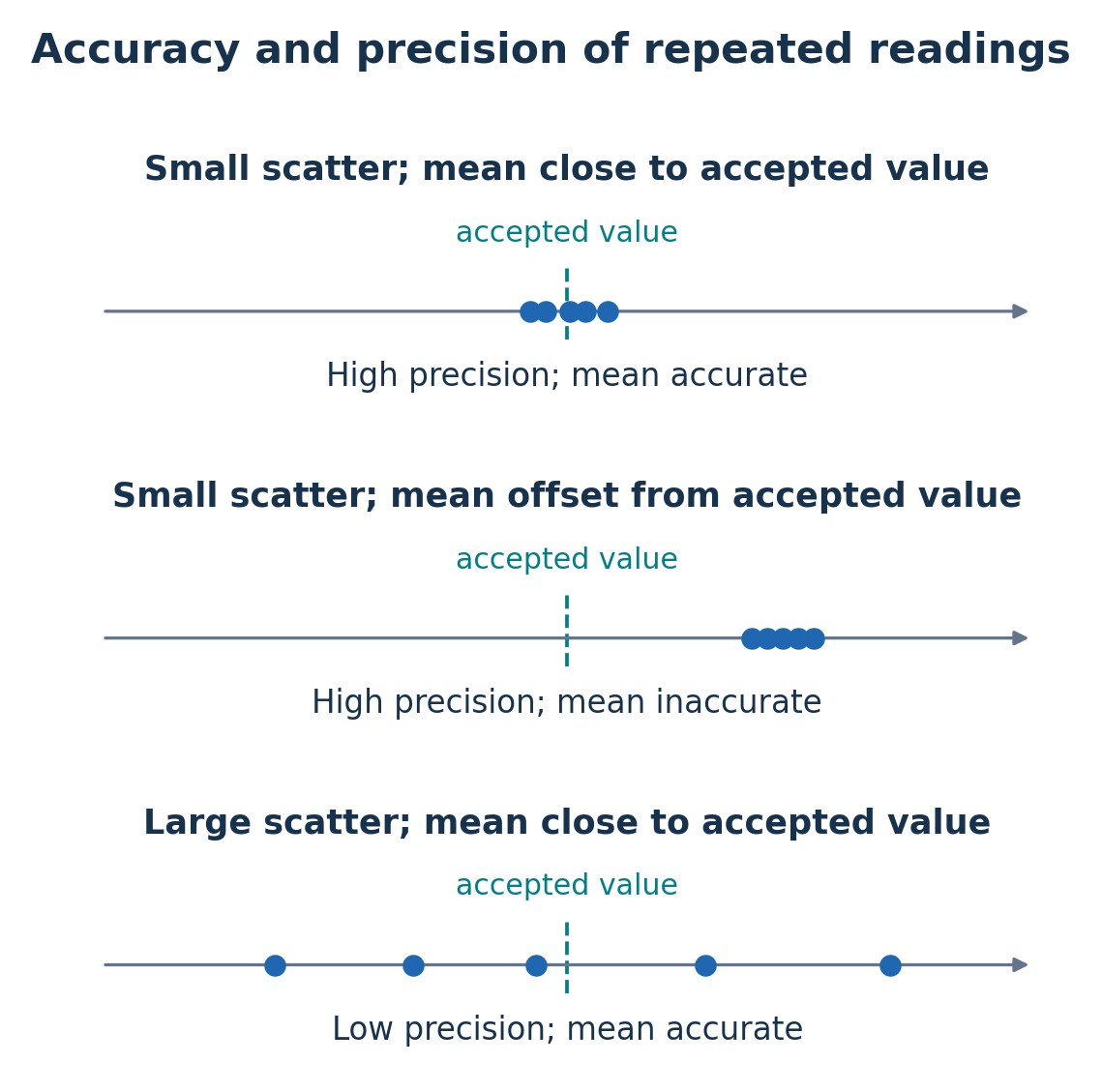
An error is a difference between a measured value and the true value; usually the true value is unknown. An uncertainty states the reasonable range associated with a measurement. Avoid describing an uncertainty as a known mistake. The instrument’s resolution, reading method and repeat-to-repeat variation can all contribute.A systematic error shifts measurements in a consistent way, so averaging repeated readings does not remove it. Examples include a balance with an uncorrected zero offset, a wrongly calibrated scale, or a timing method that always starts late. A systematic error need not be a constant offset; an incorrect scale factor can make the error increase with the reading.A zero error occurs when an instrument gives a non-zero reading for a true zero input. If a closed micrometer reads +0.03 mm, subtract 0.03 mm from subsequent readings. If it reads −0.02 mm, add 0.02 mm. Check the zero before and after measurements, and use an independent calibration or improved method to tackle other systematic errors.Random errors produce unpredictable scatter on either side of a central value, for example changes in reaction time or small fluctuations of a sensor reading. Repeat independent measurements and use their mean to reduce the effect of random variation on the estimated value. Record the spread as evidence of uncertainty; do not simply discard inconvenient readings. Investigate suspected anomalies and repeat them where possible.Precision concerns how tightly repeated measurements cluster, or the smallness of their uncertainty. Accuracy concerns closeness to the true or accepted value. A tightly grouped set with a zero offset is precise but inaccurate. An average can be close to an accepted value even when individual readings have large scatter. More decimal places do not automatically mean greater accuracy.Read analogue scales with the eye perpendicular to the scale to reduce parallax. For a repeated length measured from two scale readings, account for uncertainty in both end positions. Digital display resolution is a starting point, not a guarantee that the total experimental uncertainty is only one last-place digit.
A mean close to the accepted value does not mean every individual reading is accurate. Original RevisionTown diagram. Open full-size diagram
Combining uncertainties and reporting results
Write a measured value as x ± Δx, where Δx is the absolute uncertainty in the same units as x. Fractional uncertainty is Δx/|x|; percentage uncertainty is 100Δx/|x|. The AS treatment uses simple worst-case addition. It does not combine independent uncertainties by taking a square root of the sum of squares.
For q = a + b or q = a − b, add absolute uncertainties: Δq = Δa + Δb. Subtraction does not cancel uncertainty.
For q = ab or q = a/b, add fractional or percentage uncertainties: Δq/|q| = Δa/|a| + Δb/|b|.
For a power q = an, multiply fractional uncertainty by |n|. For q = a2/b, add 2Δa/|a| and Δb/|b|.
An exact numerical constant contributes no uncertainty. Apply uncertainty only to measured quantities or to constants whose uncertainty matters in the question.
Worked example: a difference
Two positions are (28.4 ± 0.1) cm and (12.6 ± 0.1) cm. Their separation is 15.8 cm with uncertainty 0.2 cm. The percentage uncertainty is (0.2/15.8) × 100 = 1.27%, approximately 1.3%. A small difference between two large readings can have a large percentage uncertainty.
Worked example: density
A cylinder has mass (84.0 ± 0.2) g, radius (1.20 ± 0.01) cm and height (3.00 ± 0.02) cm. Its density is 84.0/(π × 1.202 × 3.00) = 6.189 g cm−3. Percentage uncertainty = 100(0.2/84.0 + 2 × 0.01/1.20 + 0.02/3.00) = 2.57%. Absolute uncertainty = 0.0257 × 6.189 = 0.159 g cm−3. A suitable final report is (6.19 ± 0.16) g cm−3.Reducing the largest fractional contribution usually improves the result most. Here radius measurement contributes about 1.67%, much more than the mass contribution of about 0.24%. A better radius measurement is therefore more useful than an even more sensitive balance.
Vectors, resultants and perpendicular components
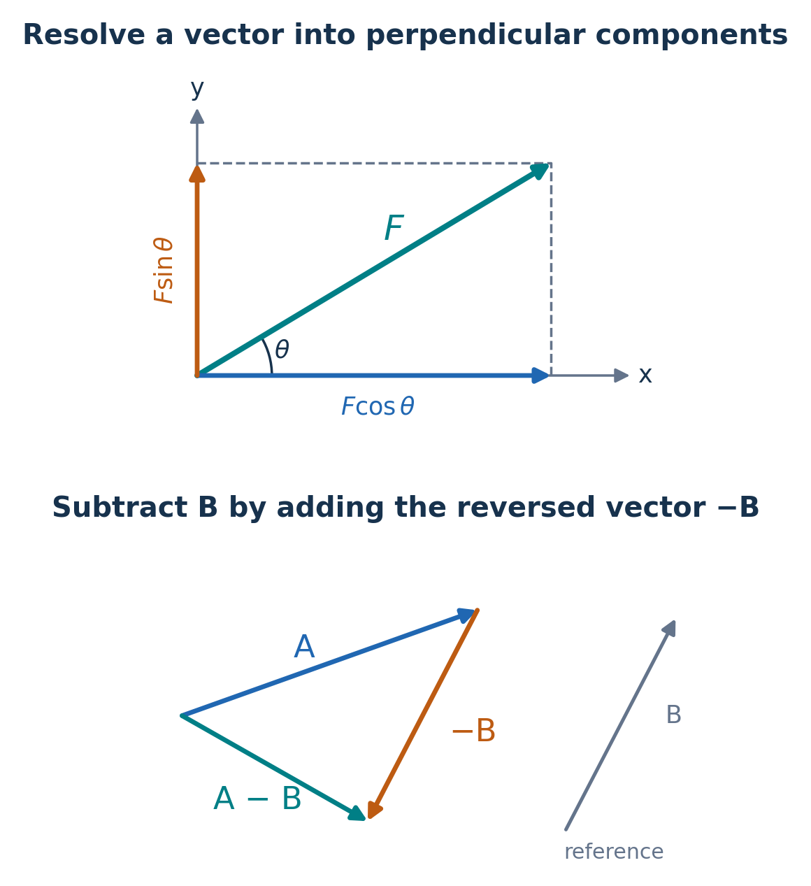
A scalar has magnitude only: mass, time, distance, speed, energy, density and temperature are examples. A vector also has direction: displacement, velocity, acceleration, force and momentum are examples. A negative component indicates a direction opposite to the selected positive axis; it does not mean that the vector’s magnitude is negative.Draw a vector as an arrow whose length represents its magnitude and whose head shows its direction. To add coplanar vectors geometrically, use a consistent scale and place the second arrow’s tail at the first arrow’s head without rotating either arrow. The resultant runs from the first tail to the last head. A parallelogram construction gives the same sum. To subtract B from A, add the reversed vector −B.Choose perpendicular x and y axes. If a vector F makes angle θ anticlockwise from the positive x direction, its components are Fx = F cos θ and Fy = F sin θ. If the angle is measured from the y axis, the roles of sine and cosine change. Sketch the triangle rather than memorising an angle-free rule.Add components separately: Rx = Ax + Bx and Ry = Ay + By. The magnitude is √(Rx2 + Ry2). The ratio Ry/Rx gives tan θ, but signs determine the quadrant. State a clear direction such as “37° north of west” instead of an unexplained calculator angle.
Worked example: a change of velocity
A boat’s initial velocity is 6.0 m s−1 east and its final velocity is 8.0 m s−1 north. Taking east and north as positive, Δv = v − u = (−6.0, +8.0) m s−1. Its magnitude is 10 m s−1, directed 53.1° north of west. The change of speed is only +2.0 m s−1; this is a different quantity from change of velocity.
A force F resolved into F cos theta along positive x and F sin theta along positive y. In a separate head-to-tail sketch, A is followed by minus B and the resultant is A minus B. Original RevisionTown diagram. Open full-size diagram
Check your understanding
Does a correct unit check prove an equation is correct?No. Matching units are necessary, but cannot check a dimensionless factor, the sign, or the physical assumptions.Will averaging remove a zero error?No. Correct the offset or calibrate the instrument. Repetition reduces the effect of random variation on the mean.When subtracting readings, should their uncertainties also be subtracted?No. The prescribed worst-case rule adds absolute uncertainties for both sums and differences.Is change of velocity simply final speed minus initial speed?Only for suitably signed motion on one axis. In general subtract the velocity vectors, including their directions.
The PDF contains the full unit practice set. Reveal an answer only after you have committed to a method.
U1-Q1 · 5 marks
A student writes “a laboratory bench has length 1.8” and estimates a 600 m walk to take 2 s. (a) Explain what is missing from the length report. (b) Using a walking speed of about 1.5 m s−1, estimate a sensible journey time. (c) State one reason the time should be treated as an estimate.Show the worked answer to U1-Q1
(a) A unit is required; for example, 1.8 m supplies both magnitude and unit. (b) t = 600/1.5 = 400 s ≈ 6.7 min. The proposed 2 s would require 300 m s−1, far above walking speed. (c) Walking speed varies, and the route distance may itself be approximate. Credit a clear assumption rather than unjustified precision.
U1-Q7 · 5 marks
The front and rear of an object are read as (18.2 ± 0.1) cm and (42.6 ± 0.1) cm on a ruler. Calculate its length, absolute uncertainty and percentage uncertainty. Explain why subtracting the readings does not justify subtracting their uncertainties.Show the worked answer to U1-Q7
Length = 42.6 − 18.2 = 24.4 cm. Worst-case absolute uncertainty = 0.1 + 0.1 = 0.2 cm. Percentage uncertainty = 100 × 0.2/24.4 = 0.820% ≈ 0.8%. Report (24.4 ± 0.2) cm. The two readings may err in opposite directions, making their difference too large or too small; uncertainty does not cancel merely because readings are subtracted.
U1-Q13 · 3 marks
Diagnostic multiple choice. Which conversion is correct? A: 2.0 cm2 = 2.0 × 10⁻² m2. B: 2.0 cm2 = 2.0 × 10⁻⁴ m2. C: 2.0 cm2 = 2.0 × 10² m2. D: 2.0 cm2 = 4.0 × 10⁻⁴ m2. Choose one option and explain the distractors.Show the worked answer to U1-Q13
Correct option: B. The unit conversion factor is squared: 2.0 cm2 = 2.0(10−2 m)2 = 2.0 × 10⁻⁴ m2. A applies a length conversion to an area. C reverses the conversion direction and fails to square it. D squares the numerical area value 2.0 unnecessarily; only the conversion of the centimetre inside cm2 is squared.
Distance is the total path length travelled and is a scalar. Displacement is the change of position from a chosen starting point, with a direction, and is a vector. A displacement can be negative along a chosen axis; distance travelled cannot decrease as a journey continues.Average speed = total distance/total time. Average velocity = displacement/time interval. Instantaneous speed is the magnitude of instantaneous velocity. Acceleration is the rate of change of velocity: average acceleration = (v − u)/Δt. Displacement and distance have unit m, speed and velocity m s−1, and acceleration m s−2. Always define the positive direction before inserting signed values.A negative velocity means motion in the negative direction. A negative acceleration means that velocity is changing towards the negative direction. It need not mean slowing down: an object with both negative velocity and negative acceleration increases its speed. Speed decreases when the acceleration component is opposite to the velocity.
Worked example: an out-and-back walk
A walker travels 240 m east and then 90 m west in 220 s. Taking east as positive, displacement is 240 − 90 = 150 m, whereas distance is 240 + 90 = 330 m. Average velocity is 150/220 = 0.682 m s−1 east; average speed is 330/220 = 1.50 m s−1. Do not average the two leg speeds unless the time weighting makes that valid.At a turning point in straight-line motion the instantaneous velocity is zero. The acceleration may still be non-zero, as for a ball at the top of a vertical throw. Being at rest at one instant does not establish equilibrium or zero acceleration.
Read motion graphs using gradients and areas
On a displacement–time graph, the gradient gives velocity. A straight sloping line shows constant velocity; a horizontal line shows rest. A steeper positive gradient means a larger positive velocity. A negative gradient means motion in the negative direction. For a curve, draw a tangent at the required time and use two well-separated points on that tangent to calculate its gradient. A chord gives average velocity over an interval, not usually instantaneous velocity at either end.On a distance–time graph, gradient gives speed. Since accumulated distance cannot fall, a descending line cannot represent total distance travelled. A displacement–time graph can descend. The distinction matters whenever an object reverses direction.On a velocity–time graph, gradient gives acceleration: a = Δv/Δt. A horizontal line can show non-zero constant velocity but always shows zero acceleration. A curved line indicates changing acceleration. The signed area between the graph and the time axis is displacement: areas above the axis are positive and those below are negative. Total distance is found by adding the magnitudes of those areas.On a speed–time graph, area gives distance. Its gradient gives the rate of change of speed, which does not by itself describe acceleration when direction changes. On an acceleration–time graph, signed area gives change of velocity; add that change to the initial velocity. A constant positive acceleration therefore gives a horizontal acceleration graph, a straight rising velocity graph and a displacement–time graph whose gradient increases with time. Its gradient may be negative, zero or positive depending on the initial velocity.
Worked example: a velocity reversal
A trolley’s velocity falls uniformly from +6.0 m s−1 at t = 0 to −2.0 m s−1 at t = 4.0 s. Acceleration = (−2.0 − 6.0)/4.0 = −2.0 m s−2. The trolley stops momentarily at 3.0 s. Positive area is ½ × 3.0 × 6.0 = 9.0 m; negative area is −½ × 1.0 × 2.0 = −1.0 m. Displacement is 8.0 m and distance is 10.0 m.Label axes with quantities and units, choose readable scales, and retain the physical meaning of signs. Areas have the product of the axis units, while gradients have the quotient. These unit checks often expose choosing the wrong graphical method.
Derive and use constant-acceleration equations
The standard equations require constant acceleration, motion resolved along a fixed straight axis and consistent sign conventions. Define u as velocity at the start of the interval, v as velocity at its end, a as the constant acceleration, t as elapsed time and s as displacement during that interval. Initial position is separate: final position = initial position + s.From a = (v − u)/t, rearrange to obtain v = u + at. Since velocity changes uniformly, its mean value is (u + v)/2. The area under the straight velocity–time line is consequently s = ½(u + v)t. Substituting v = u + at gives s = ut + ½at2. Alternatively, substitute u = v − at to give s = vt − ½at2.Eliminate t between s = ½(u + v)t and t = (v − u)/a. This gives 2as = (u + v)(v − u) = v2 − u2, hence v2 = u2 + 2as. The form with squares loses the sign of the final velocity, so recover direction from the physical situation rather than automatically selecting a positive root.
List the known and required quantities with signs and units.
Choose the equation that excludes an unneeded unknown.
Use one time origin and one axis for that calculation.
Check whether acceleration really is constant; split a journey into separate stages if needed.
Worked example: braking
A vehicle moving at +18.0 m s−1 stops with acceleration −3.00 m s−2. From v = u + at, t = (0 − 18.0)/(−3.00) = 6.00 s. From v2 = u2 + 2as, s = (0 − 18.02)/(−6.00) = 54.0 m. The displacement is positive because the vehicle still moves forwards while slowing. The model should not be extended beyond stopping unless the forces then cause reverse motion.
Free fall and vertical throws
Free fall means motion under gravity alone. In a uniform gravitational field close to Earth’s surface, acceleration is approximately g = 9.81 m s−2 vertically downward. The model neglects air resistance. Mass does not appear in the kinematic equations for this motion, so objects released with the same initial conditions have the same ideal trajectory.If upward is positive, a = −g throughout the flight. An upward-moving object slows, reaches zero vertical velocity, and then accelerates downwards. Its acceleration does not become zero at the top and does not change sign there. If downward is positive, a = +g; either convention works if used consistently.
Worked example: reaching a height
A ball is thrown vertically upwards at 14.0 m s−1. With upward positive, its maximum height above release satisfies 0 = 14.02 − 2gh, so h = 196/19.62 = 9.99 m. Time to the top is 14.0/9.81 = 1.43 s. It returns to its launch height after 2.85 s with velocity −14.0 m s−1. The equal rise and fall times apply here because the launch and return heights are equal and air resistance is neglected.When asked for a time at an intermediate height, a quadratic can have two positive roots: one for upward travel and one for downward travel. Select the root that matches the event, or state both if both are physically relevant. The constant-g approximation becomes less appropriate over distances comparable with Earth’s radius.
Measure the acceleration of free fall
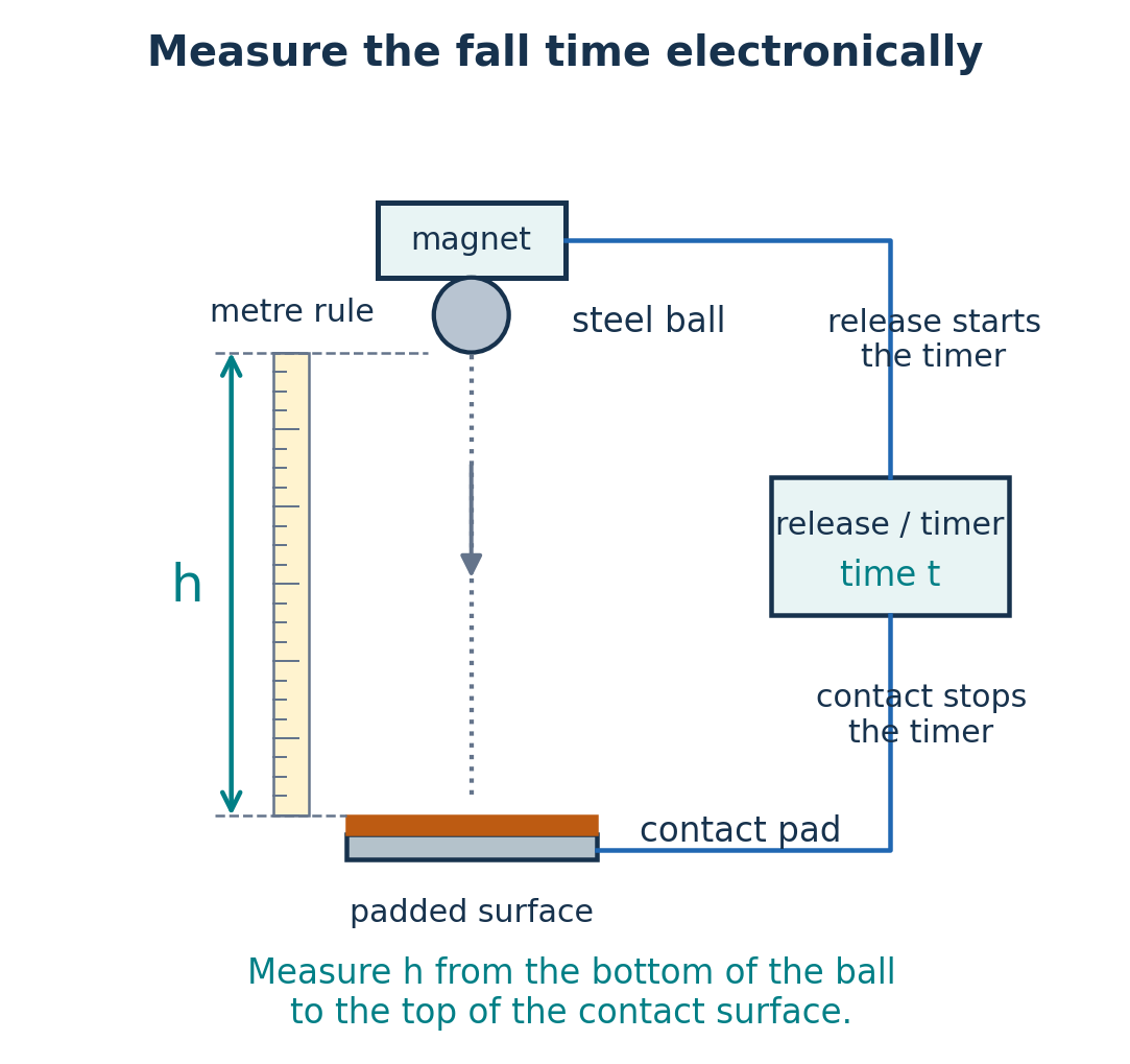
A suitable experiment measures the motion of a falling object with electronic timing, reducing the large fractional uncertainty associated with hand timing a short fall. One method releases a small steel ball from an electromagnet. The release circuit starts a timer and a contact pad stops it when the ball reaches the lower level. Use a tray or padding to catch the ball, secure the apparatus and keep feet clear.Measure the vertical distance h travelled by a fixed point on the ball from release to first contact. For example, use the ball’s bottom surface in both positions; measuring from its centre at release to the contact surface adds a systematic height error. Release without an initial push. Use a compact dense ball and a moderate drop height so air resistance is relatively small.Repeat the time measurement for each of several heights. Record the scatter, find a mean time and calculate t2. For release from rest, h = ½gt2, so a graph of h against t2 should be approximately straight with gradient g/2. Thus g = 2 × gradient. Use a large triangle on the best-fit line, not two arbitrary raw data points. Repeated readings reduce random timing variation, but do not remove a fixed electronic release delay or an incorrect distance zero. Investigate a non-zero intercept rather than automatically forcing the fit through the origin.A light-gate alternative measures speeds at two vertical positions. A short known interrupting length L gives speed approximately L/Δt while passing a gate. Use g = (v − u)/ΔT with the interval between the speed measurements, or plot v2 against fall distance to obtain gradient 2g. The speed estimate is an interval average, so a short interrupting length and appropriate timing positions matter.Estimate uncertainty from distance resolution, timing uncertainty and repeat scatter. For a single release, g = 2h/t2 gives Δg/g ≈ Δh/h + 2Δt/t. A larger safe fall height often reduces percentage distance and timing uncertainty, but do not increase it so much that drag or apparatus limitations dominate.
An electromagnet releases a steel ball onto a padded contact pad. The release and contact operate an electronic timer. Height h is measured using a metre rule from the bottom of the released ball to the top of the contact surface. Original RevisionTown diagram. Open full-size diagram
A projectile moving without air resistance has constant horizontal velocity and constant downward vertical acceleration. Resolve the initial velocity, then analyse the two directions separately using the same elapsed time. The horizontal and vertical motions do not exchange acceleration; gravity changes the vertical component only.Taking x horizontally and y upward, an initial speed u at angle θ above horizontal gives ux = u cos θ and uy = u sin θ. Relative to the launch point, x = u cos θ × t, y = u sin θ × t − ½gt2, vx = u cos θ and vy = u sin θ − gt. Find resultant speed from √(vx2 + vy2) and direction from the component ratio, accounting for signs.Eliminating t gives y = x tan θ − gx2/(2u2 cos2 θ), a parabolic trajectory. For launch and landing at the same height, setting y = 0 gives flight time 2u sin θ/g and horizontal range u2 sin 2θ/g. These shortcuts assume equal heights; use the component equations for an elevated launch or landing.
Worked example: leaving a ledge horizontally
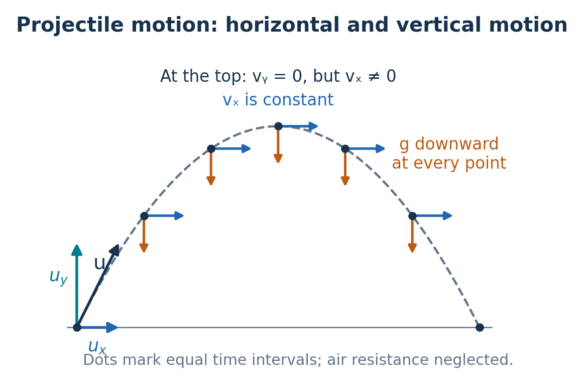
A ball leaves a ledge 5.00 m above level ground with horizontal speed 4.00 m s−1. Downward displacement gives 5.00 = ½gt2, so t = 1.01 s. Horizontal range is 4.00t = 4.04 m. Its downward velocity just before impact is gt = 9.90 m s−1, and speed is √(4.002 + 9.902) = 10.7 m s−1. A ball simply dropped from the same ledge at the same instant lands simultaneously in this ideal model.At the highest point of an angled projectile, vy = 0 but vx is generally non-zero. Its velocity is horizontal and its acceleration is still vertically downward.
A parabolic projectile trajectory has equal horizontal spacing between equal-time markers. Blue horizontal velocity arrows have equal lengths, and orange gravitational acceleration arrows always point down. At the highest point vertical velocity is zero but horizontal velocity is not. Original RevisionTown diagram. Open full-size diagram
Check your understanding
Does negative acceleration always mean slowing down?No. Speed increases when velocity and acceleration point in the same direction, including when both are negative.Is the area below a velocity–time graph always distance?Signed area gives displacement. Add the magnitudes of positive and negative areas for distance.Is acceleration zero at the top of a projectile’s flight?No. The vertical velocity is momentarily zero, while gravitational acceleration remains downward.Can the equal-height range formula be used for a projectile launched from a cliff?Not generally. Solve vertical motion for the actual landing height, then use horizontal velocity and the shared flight time.
The PDF contains the full unit practice set. Reveal an answer only after you have committed to a method.
U2-Q1 · 6 marks
A student runs 40 m east, then 30 m west, in 14 s. (a) Find distance and displacement. (b) Find average speed and average velocity. (c) Explain why an object travelling west can have an eastward acceleration.Show the worked answer to U2-Q1
(a) Distance = 40 + 30 = 70 m; displacement = 40 − 30 = 10 m east. (b) Average speed = 70/14 = 5.0 m s−1; average velocity = 10/14 = 0.714 m s−1 east. (c) Eastward acceleration changes velocity towards the east; a westward-moving object initially slows until it stops, and may subsequently reverse.
U2-Q7 · 5 marks
A small dense sphere is dropped from rest 45.0 m above the ground. Assuming negligible air resistance and g = 9.81 m s−2, calculate the fall time and impact speed. State one physical reason the measured result might depart from this model.Show the worked answer to U2-Q7
Taking downward positive, 45.0 = ½(9.81)t2 gives t = √(90.0/9.81) = 3.03 s. Impact speed = gt = 29.7 m s−1, also √(2gh). Air resistance produces an upward force, reducing downward acceleration below g and tending to increase the fall time and reduce impact speed compared with the ideal model.
U2-Q13 · 3 marks
Diagnostic multiple choice. A straight velocity–time line slopes from +4 m s−1 at 0 s to −4 m s−1 at 4 s. Which pair gives displacement and distance travelled? A: 0 m and 0 m. B: 8 m and 8 m. C: 0 m and 8 m. D: −8 m and 0 m. Choose one option and explain the distractors.Show the worked answer to U2-Q13
Correct option: C. Velocity reaches zero at 2 s. Each triangular area has magnitude ½ × 2 × 4 = 4 m. Signed areas cancel, giving displacement 0 m; their magnitudes add to distance 8 m. A confuses returning to the initial position with no travel. B adds area magnitudes for displacement as well as distance. D uses a negative distance-related result and ignores the positive part of the graph.
Mass measures an object’s inertia: its resistance to a change of velocity. With the same resultant force, a larger mass has a smaller acceleration. Mass is a scalar measured in kilograms. It is not a force and does not depend on the local gravitational field.In an inertial reference frame, Newton’s first law states that an object maintains a constant velocity, including rest, unless acted on by a non-zero resultant external force. It does not require a forward force to maintain motion. In ordinary life, a moving object often slows because friction or drag supplies a backward resultant force.Newton’s second law relates resultant force to the rate of change of momentum. For constant mass, Fresultant = ma. In components, ΣFx = max and ΣFy = may. Resultant force and acceleration always point in the same direction; velocity need not point that way. When a vehicle moving forward brakes, velocity is forward while acceleration and resultant force are backward.Newton’s third law states that when one body exerts a force on another, the second exerts a force of equal magnitude and opposite direction on the first. The forces have the same interaction type, act on different bodies and exist simultaneously. They therefore do not cancel on the free-body diagram of one object. A foot pushes the ground backwards and the ground pushes the foot forwards.To solve a force problem, select the object or system, draw only forces acting on it, choose axes, and calculate the vector resultant. Do not label a single applied force “ma” unless all other forces along that direction have been accounted for. Forces on connected bodies may be internal to a combined system but external to each separate body.
Worked example: an accelerating crate
A 12.0 kg crate is pulled horizontally by 54.0 N against 18.0 N resistance. Its resultant is 54.0 − 18.0 = 36.0 N, giving a = 36.0/12.0 = 3.00 m s−2 in the pulling direction. If the resistance becomes 54.0 N, the acceleration is zero; the crate may still move at a non-zero constant velocity.
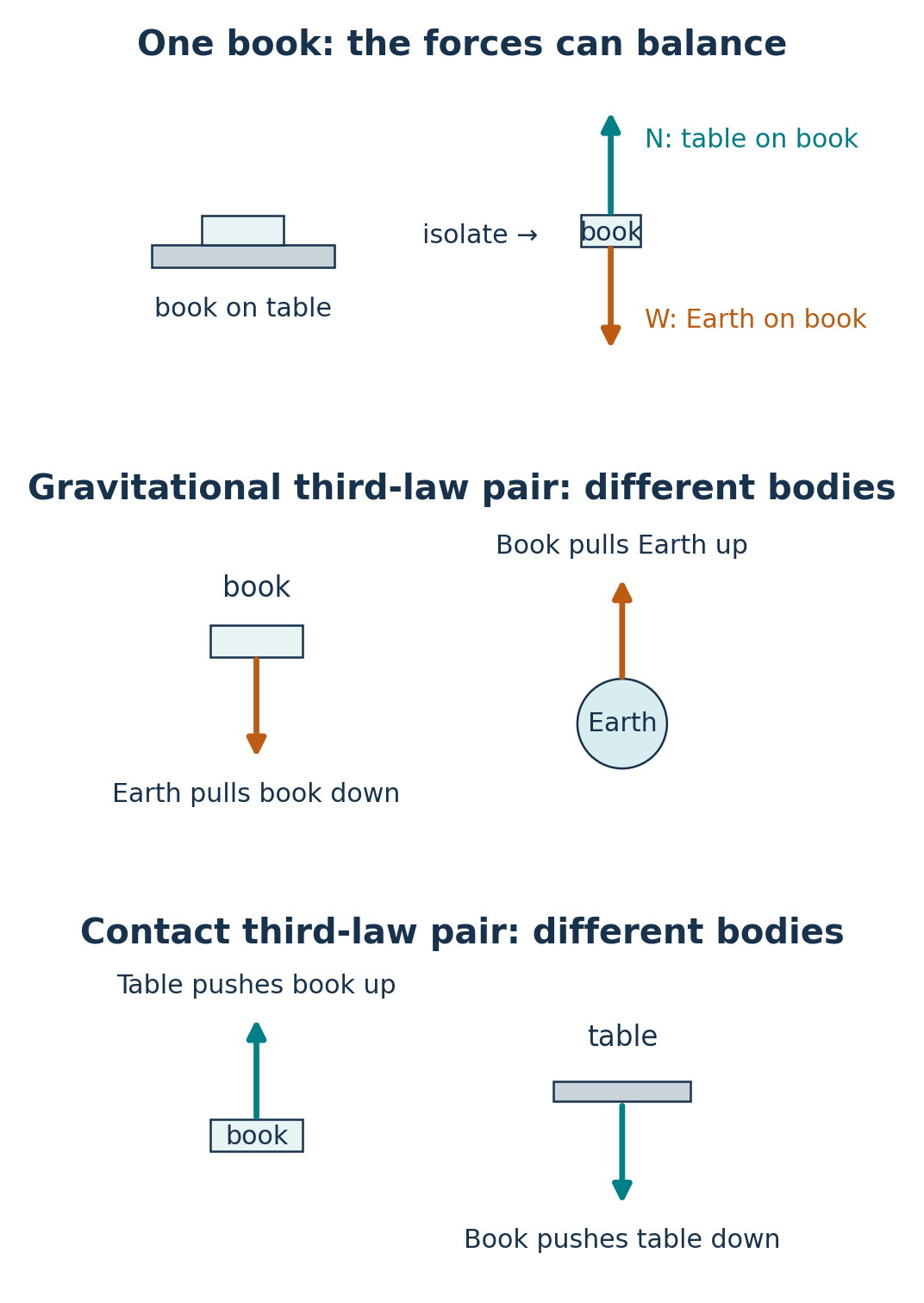
The book-only free-body diagram has an upward table force and downward Earth force. The gravitational third-law pair acts separately on the book and Earth; the contact third-law pair acts separately on the book and table. Equal arrow lengths within each pair indicate equal force magnitudes. Original RevisionTown diagram. Open full-size diagram
Weight and support forces
Weight is the gravitational force acting on a mass. In a field where the acceleration of free fall is g, W = mg. Its unit is the newton and its direction is the local downward direction. Numerically, gravitational field strength in N kg−1 equals free-fall acceleration in m s−2. Near Earth’s surface, use the stated value or approximately 9.81.A normal contact force is exerted perpendicular to a surface. Tension acts along a stretched string. Neither is automatically equal to weight. Equality follows only when the other forces and acceleration make it so. On a horizontal floor with no vertical acceleration and no additional vertical forces, N − mg = 0 and hence N = mg.The upward normal force on a book and the downward weight of that book can balance, but they are not a Newton’s-third-law pair because both act on the book. The partner to the table’s upward force on the book is the book’s downward force on the table. The partner to Earth’s gravitational force on the book is the book’s gravitational force on Earth.
Worked example: a lift scale
A 50.0 kg passenger accelerates upward at 1.20 m s−2. With upward positive, N − mg = ma, so N = 50.0(9.81 + 1.20) = 550.5 N, about 551 N. If the acceleration is downward at 1.20 m s−2, N = 50.0(9.81 − 1.20) = 430.5 N. A scale measures the support force, not the gravitational force directly. In ideal free fall, N = 0 although the passenger’s weight remains mg.
Momentum, force and impulse
Linear momentum is p = mv. It is a vector in the velocity direction, with unit kg m s−1, equivalent to N s. Use signed velocities or components: a rebound can produce a much larger change of momentum than a stop from the same initial speed.Resultant force is the rate of change of momentum. Over a finite interval, average resultant force = Δp/Δt. Instantaneous force corresponds to the gradient of a momentum–time graph. For constant mass, Δp/Δt = mΔv/Δt, recovering F = ma.Impulse is the change of momentum delivered by a resultant force: FaverageΔt = Δp. It is also the signed area under a force–time graph. A triangular force pulse with peak F and duration Δt has impulse ½FΔt. Distinguish the peak from the average force. Increasing the collision time for the same momentum change reduces average force, explaining how cushioning helps.
Worked example: a rebounding ball
A 0.200 kg ball moving at +7.0 m s−1 rebounds at −5.0 m s−1 after 0.040 s contact with a wall. Its change of momentum is 0.200(−5.0 − 7.0) = −2.4 kg m s−1. Average resultant force is −2.4/0.040 = −60 N, directed away from the wall. Subtracting the speeds would give the wrong change because it ignores reversal.If other forces matter during the contact, the force inferred from Δp/Δt is their resultant with the contact force. For a very short horizontal collision, the horizontal wall force can often be identified directly, while vertical weight has negligible effect on horizontal momentum.
Friction, drag and terminal velocity
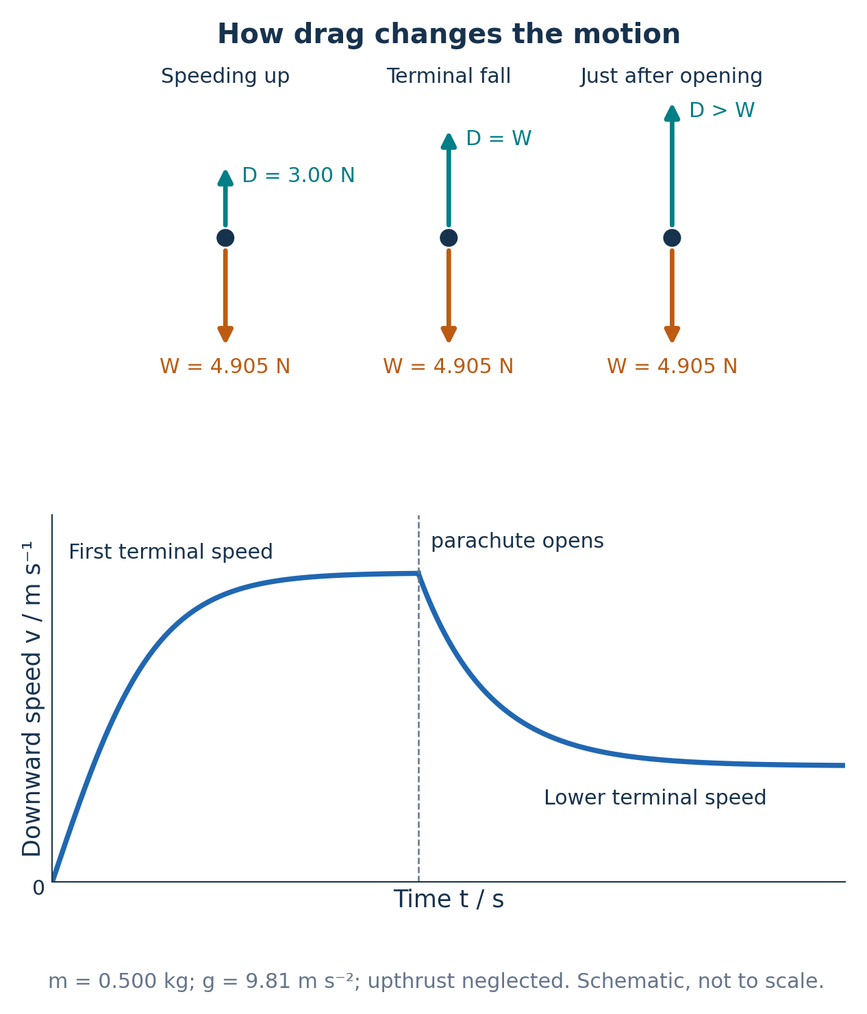
Friction opposes relative sliding, or the tendency to slide, between contacting surfaces. Static friction can adjust to the force required to prevent slipping up to a limiting value; it is not necessarily a fixed force. Friction can propel an object, as with a walking person, so “friction always opposes the object’s velocity” is an unreliable rule.Viscous resistance and air resistance oppose motion relative to the surrounding fluid. Their magnitude normally increases with relative speed. A qualitative increasing-drag model is sufficient here; no coefficient-of-friction or viscosity formula is needed. Shape, exposed area and the fluid can affect resistance.In the following air-resistance examples, neglect upthrust (buoyancy). If it is significant, terminal downward motion instead requires W = D + U, where U is upthrust. For an object released from rest in air, downward weight is initially larger than upward drag, which is initially zero in still air. It accelerates downward. As speed rises, drag increases and the downward resultant W − D decreases, so the downward acceleration decreases. Eventually drag equals weight and acceleration becomes zero. The object continues falling at terminal velocity: constant velocity with balanced forces, not zero velocity.A downward speed–time graph starts with a large positive gradient that gradually falls towards zero and approaches a horizontal line. The acceleration–time graph begins near g and decreases towards zero. If a parachute opens, the larger drag can initially exceed weight; the falling person then accelerates upward while still moving downward, so slows. As speed decreases, drag decreases until it again equals weight at a lower terminal speed.For an object projected vertically upward, weight and drag both act downward during ascent, so the downward acceleration can exceed g. At the highest point, drag is momentarily zero in still air but weight is not. During descent, drag is upward. The upward and downward motions are no longer symmetric.Terminal motion also occurs horizontally: if a vehicle’s driving force balances speed-dependent resistance, its acceleration becomes zero. A larger driving force initially makes a forward resultant, and speed increases until resistance balances the new force, if such a steady state is possible.
Teaching diagram only. The speed is continuous at opening; its gradient changes abruptly. Original RevisionTown diagram. Open full-size diagram
Choose a system before conserving momentum
The total vector momentum of a system remains constant when the resultant external force on that system is zero. During a brief interaction, momentum may be treated as conserved when the external impulse is negligible compared with the momentum exchanged. State this condition and identify the system, rather than applying conservation merely because a collision occurs.During an interaction, forces between the bodies are equal and opposite. Their impulses cancel in the total momentum change of the combined system, so internal forces cannot change its total momentum. They can transfer momentum between individual objects. If a wall, support or Earth exerts a significant external impulse on a chosen smaller system, include the relevant interacting body in a larger system or account for that impulse explicitly.Momentum conservation is a vector statement: total px before = total px after, and independently total py before = total py after. Add signed components, not just momentum magnitudes.An elastic collision conserves total kinetic energy as well as momentum. In an inelastic collision, some initial kinetic energy becomes internal energy, sound or deformation. A completely inelastic collision is the special case where objects remain together. Momentum can be conserved even when kinetic energy is not. Total energy is still conserved when all forms are included. Explosions can increase kinetic energy by transferring stored internal energy; they do not create energy.Always compare total kinetic energy, Σ½mv2, rather than each body’s kinetic energy. One object can gain kinetic energy at another’s expense in an elastic collision. In a completely inelastic collision use the combined mass and common final velocity, then calculate the kinetic-energy change separately.
One-dimensional collisions and recoil
For two bodies on a line with negligible external impulse, m1u1 + m2u2 = m1v1 + m2v2. Select one positive direction for all four velocities. If the bodies stick, v1 = v2 = v and the right side becomes (m1 + m2)v.For a one-dimensional elastic collision, the relative speed of approach equals the relative speed of separation. When body 1 approaches body 2 from behind, write u1 − u2 = v2 − v1. This relation, together with momentum conservation, determines both final velocities. It must not be imposed on an inelastic collision. Use full vector momentum and kinetic-energy conservation for general two-dimensional elastic interactions.
Worked example: sticking trolleys
A 0.80 kg trolley moving at +3.0 m s−1 sticks to a stationary 0.40 kg trolley. Total initial momentum = 2.4 kg m s−1, so common velocity = 2.4/1.20 = +2.0 m s−1. Initial kinetic energy = ½(0.80)(3.0)2 = 3.6 J. Final kinetic energy = ½(1.20)(2.0)2 = 2.4 J. The 1.2 J decrease is compatible with conserved momentum because the quantities obey different conservation conditions.For recoil from rest, total initial momentum is zero. The separated parts therefore have equal and opposite momenta, not generally equal speeds. If a light fragment moves quickly one way, a heavy fragment moves more slowly the other way. The kinetic energy comes from energy stored before separation.
Two-dimensional interactions
Draw axes and resolve every initial and final momentum along both. There are two independent conservation equations. If two objects stick, first calculate the common velocity components and then reconstruct its magnitude and direction. Do not equate scalar totals of momentum magnitudes: two equal opposite momenta sum to zero.
Worked example: a two-dimensional inelastic collision
A 2.0 kg cart moving east at 3.0 m s−1 meets and sticks to a 1.0 kg cart moving north at 4.0 m s−1 on a level low-friction surface. External horizontal impulse is negligible. Initial momentum components are (6.0, 4.0) kg m s−1. Dividing each by total mass 3.0 kg gives final velocity (2.0, 1.333) m s−1. Its magnitude is 2.40 m s−1, at 33.7° north of east. Initial kinetic energy is 9.0 + 8.0 = 17.0 J; final kinetic energy is ½(3.0)(2.02 + 1.3332) = 8.67 J, so 8.33 J is transferred to other forms.
Worked example: a two-dimensional elastic collision
A 0.200 kg puck initially moves at 6.00 m s−1 along x and strikes an identical stationary puck. Afterwards the first travels at 3√3 m s−1 at +30°, and the second at 3.00 m s−1 at −60°. Their velocity components are (4.50, 2.598) and (1.50, −2.598) m s−1. Total momentum is therefore 0.200(6.00, 0), unchanged. Final kinetic energy is ½(0.200)(27 + 9) = 3.60 J, equal to the initial ½(0.200)(6.00)2. Checking both component equations and energy establishes the claimed elastic outcome.
Check your understanding
Are weight and normal reaction a Newton’s-third-law pair?No. They act on the same object. Each has a partner acting on a different body.Does terminal velocity mean no forces act?No. The forces balance, so resultant force and acceleration are zero while velocity can remain non-zero.Is momentum automatically conserved for any selected object during a collision?No. Define the system and check its external impulse. Internal impulses cancel only when both interacting bodies are included.Can momentum be conserved when kinetic energy decreases?Yes. An inelastic isolated interaction conserves total momentum while converting some kinetic energy into internal energy, sound or deformation.
The PDF contains the full unit practice set. Reveal an answer only after you have committed to a method.
U3-Q1 · 6 marks
A 40.0 kg trolley is pushed horizontally with 180 N while resistance is 60 N. (a) Find its acceleration. (b) State how acceleration changes if the mass doubles but both forces remain the same. (c) State Newton’s first law and explain what happens when the pushing force becomes 60 N while the trolley is moving.Show the worked answer to U3-Q1
(a) Resultant = 180 − 60 = 120 N forwards; a = 120/40.0 = 3.00 m s−2. (b) Acceleration halves to 1.50 m s−2; the larger mass has greater inertia. (c) With zero resultant external force, a body stays at rest or moves at constant velocity. A 60 N push balances 60 N resistance, so the moving trolley continues at constant velocity in this model.
U3-Q7 · 8 marks
On a low-friction track a 0.600 kg cart moving at +5.00 m s−1 collides with a 0.400 kg cart moving at −1.00 m s−1. They stick. (a) State the momentum-conservation condition. (b) Find their final velocity. (c) Calculate the kinetic-energy decrease and explain where the energy can go.Show the worked answer to U3-Q7
(a) External impulse on the two-cart system must be negligible during the collision. (b) Initial momentum = 0.600(5.00) + 0.400(−1.00) = 2.60 kg m s−1. Total mass = 1.000 kg, so v = +2.60 m s−1. (c) Initial kinetic energy = ½(0.600)(25.0) + ½(0.400)(1.00) = 7.70 J. Final = ½(1.000)(2.60)2 = 3.38 J. Decrease = 4.32 J, transferred to deformation, internal energy and sound; momentum remains conserved.
U3-Q12 · 3 marks
Diagnostic multiple choice. Two carts stick together in a brief collision with negligible external impulse. Which statement is correct? A: Momentum and kinetic energy must both be conserved. B: Neither is conserved because the carts deform. C: Total momentum is conserved but kinetic energy may decrease. D: Each cart separately retains its original momentum. Choose one option and explain the distractors.Show the worked answer to U3-Q12
Correct option: C. Internal impulses cancel for the two-cart system, while kinetic energy can become other energy forms. A treats an inelastic collision as elastic. B confuses kinetic-energy loss with loss of total momentum. D applies system conservation to individual carts, each of which experiences a large interaction impulse and changes momentum.
The weight of an extended object can be represented by a single force acting through its centre of gravity. In a uniform gravitational field this coincides with the centre of mass. For a uniform symmetrical object, symmetry locates the centre of gravity; a non-uniform object need not have its centre of gravity at its geometric centre. The point can lie outside the material, as for a ring.For an irregular thin lamina, suspend it freely from one point and mark the vertical line indicated by a plumb line. Repeat from another point. The intersection locates its centre of gravity because the weight’s line of action must pass through the suspension point in equilibrium. Use a freely moving pivot and mark carefully to reduce practical error.The moment of a force about a point measures its turning effect: moment = force × perpendicular distance from the point to the force’s line of action. Its unit is N m. Identify clockwise or anticlockwise sense, or adopt a consistent signed convention. The lever arm is not generally the distance from the pivot to the point where the force is applied.If a force F acts at a distance r from a pivot, at angle θ to the position vector, the perpendicular distance is r sin θ, so the moment magnitude is Fr sin θ. A force directed through the pivot has zero moment even if its magnitude is large. Resolve the force or find the perpendicular distance, but do not do both and count the same sine factor twice.
Worked example: an angled push
A 30.0 N force is applied 0.250 m from a pivot at 60.0° to the lever. Moment magnitude = 30.0 × 0.250 × sin 60.0° = 6.50 N m. If the same force is applied perpendicular to the lever, its moment becomes 7.50 N m. State clockwise or anticlockwise using the diagram.An unrestrained object resting on a supporting surface begins to tip about the edge of its base when the vertical line through its centre of gravity passes outside that base. At the limiting position the line passes through the tipping edge, so weight has zero moment about that edge. A lower centre of gravity and wider base generally improve stability.
Couples and their torque
A couple consists of two equal, opposite, parallel forces acting along different lines. Their resultant force is zero, but their moments act in the same rotational sense. A couple therefore produces a turning effect without a resultant translational force. Applying two equal opposite forces along the same line produces no couple because their separation is zero.The torque of a couple is τ = Fd, where F is the magnitude of one of the forces and d is the perpendicular separation of their lines of action. It is not 2Fd when d already represents the full separation. The SI unit is N m. Although this is algebraically the same combination of units as a joule, torque is quoted as N m to distinguish its physical meaning from energy.Choose any point between the forces. If their perpendicular distances from that point are d1 and d2, their moments add to Fd1 + Fd2 = F(d1 + d2) = Fd. Taking moments about another point gives the same total. A couple’s torque does not depend on the chosen origin.
Worked example: turning a wheel
Two hands exert opposite tangential forces of 40.0 N with their lines of action separated by 0.180 m. Torque = 40.0 × 0.180 = 7.20 N m. Calculating about the centre gives two contributions of 40.0 × 0.090 = 3.60 N m, which sum to 7.20 N m.
Equilibrium, moments and force triangles
For an object in complete equilibrium, both the resultant force and resultant torque are zero. In coplanar problems, use ΣFx = 0, ΣFy = 0 and ΣM = 0. Zero resultant force alone does not prevent rotational acceleration, as a couple demonstrates. Zero resultant moment about one point alone does not guarantee translational equilibrium.The principle of moments states that, for a body in equilibrium, total clockwise moment equals total anticlockwise moment about any chosen point. Pick a convenient point, often an unknown support force’s point of application, to eliminate that force from the moment equation. Then use force balance to find any remaining unknown.
Worked example: a supported beam
A uniform 4.00 m horizontal beam weighs 200 N and is supported at both ends. A 300 N load acts 3.00 m from the left support. Weight of the beam acts at its midpoint, 2.00 m from the left. Taking moments about the left support: Rright(4.00) = 200(2.00) + 300(3.00). Hence Rright = 325 N. Vertical balance gives Rleft = 200 + 300 − 325 = 175 N. These positive answers match upward contact reactions.Three coplanar forces in equilibrium can be represented by a closed head-to-tail vector triangle. Draw each vector parallel to its actual force direction using a chosen scale. Closure means their vector sum is zero. This force triangle describes force balance; for an extended object, also check moment balance. Three non-parallel forces on a rigid object in equilibrium have lines of action meeting at one point.
Worked example: unequal cable directions
A 100 N load is held at a knot by cables sloping upward at 30° left and 60° right to the horizontal. Horizontal balance gives TLcos30° = TRcos60°. Vertical balance gives TLsin30° + TRsin60° = 100. Substituting TR = √3TL gives 2TL = 100, so TL = 50.0 N and TR = 86.6 N. These two tension vectors and the downward weight form a closed triangle.
Density and pressure in useful units
Density is mass per unit volume: ρ = m/V. Its SI unit is kg m−3. Rearranged forms are m = ρV and V = m/ρ. Density characterises the material under stated conditions, whereas mass and volume depend on how much material is present. A hollow object’s average density uses its total mass and the relevant overall volume, not automatically the density of the shell material.For a regular solid, determine volume from measured dimensions. For a cylinder, V = πr2h; for a rectangular block, V = lwh. An irregular solid can displace liquid in a measuring cylinder, provided it is fully submerged and does not dissolve or trap air. Read the meniscus consistently. For a liquid, subtract the empty container mass from the filled mass and divide by the liquid volume.Convert units before substitution. Since 1 cm3 = 10−6 m3 and 1 g = 10−3 kg, 1 g cm−3 = 1000 kg m−3. Cubing the length conversion is essential.Pressure is normal force per unit area: p = F/A for a uniform pressure over area A. Its SI unit is Pa = N m−2. A smaller contact area gives greater pressure for the same normal force. Pressure is a scalar; the force due to fluid pressure acts perpendicular to each surface, so its direction depends on that surface’s orientation.
Worked example: feet on a floor
A person exerts a total normal force of 540 N over two soles with combined area 360 cm2. The area is 0.0360 m2, so mean pressure is 540/0.0360 = 1.50 × 10⁴ Pa. Using 360 directly would fail because the area would not be in square metres.
Derive and apply hydrostatic pressure
A stationary fluid supports a pressure difference with depth because lower layers must support the weight of fluid above. Consider an imaginary vertical column of fluid with cross-sectional area A and height Δh. For a uniform-density fluid, its volume is AΔh, mass is ρAΔh and weight is ρAΔhg.The lower face experiences upward force pbottomA; the upper face experiences downward force ptopA. Horizontal pressure forces have no vertical resultant. Vertical equilibrium gives pbottomA − ptopA − ρAΔhg = 0. Dividing by A yields Δp = pbottom − ptop = ρgΔh.The derivation assumes stationary fluid, constant density over the height considered and approximately uniform g. The depth difference is vertical, not the length along a sloping tube. The result is independent of the container’s width or shape. Points at the same height in the same connected stationary fluid have equal pressure.For a liquid open to the atmosphere, absolute pressure at depth h is p = patmosphere + ρgh. Gauge pressure is the excess above atmosphere, ρgh. Decide which the question requests. For several fluid layers, add each layer’s ρgΔh. Do not use one density for the whole depth if the layers have different densities.
Worked example: a depth pressure
At 2.40 m below the surface of water of density 1000 kg m−3, the pressure increase is 1000 × 9.81 × 2.40 = 23 544 Pa = 23.5 kPa. If surface pressure is 101 kPa, absolute pressure is 124.5 kPa, approximately 125 kPa at three significant figures.A graph of pressure against depth is a straight line with gradient ρg. For gauge pressure its ideal intercept is zero; for absolute pressure its intercept is the surface pressure. A measured gradient can therefore determine an unknown liquid density by dividing by g.
Upthrust, Archimedes’ principle and floating
A submerged object experiences fluid pressure on its surface. Since pressure increases with depth, upward pressure force on a lower horizontal surface exceeds downward pressure force on an equal upper surface. Sideways pressure forces cancel in a uniform stationary fluid. Their net vertical effect is an upward force called upthrust or buoyancy.For a fully immersed rectangular block of horizontal area A and vertical height h, upthrust U = (pbottom − ptop)A = ρghA. Since Ah = V, U = ρgV. Here ρ is the fluid density and V is the displaced fluid volume, not automatically the object’s total volume. The same result extends to other shapes: the upthrust equals the weight of the displaced fluid. This is Archimedes’ principle.For partial immersion, use only the submerged volume. A larger atmospheric or surface pressure contributes equal opposing effects and does not change the net upthrust for a fixed displaced volume in an incompressible liquid. Likewise, moving a rigid fully immersed object deeper does not increase its upthrust if fluid density stays constant, even though pressures on all its surfaces increase.
Worked example: an immersed object on a string
An object has mass 0.800 kg and displaces 3.00 × 10⁻⁴ m3 of water. With ρ = 1000 kg m−3, upthrust = 1000 × 9.81 × 3.00 × 10−4 = 2.943 N. Weight is 7.848 N. For equilibrium while hanging from above, T + U = W, so T = 4.905 N. The object’s apparent weight is reduced although its gravitational weight has not changed.A freely floating object in equilibrium satisfies U = W, so ρfluidgVsubmerged = mg. For a uniform object of density ρobject, the submerged fraction is Vsubmerged/Vtotal = ρobject/ρfluid. A 600 kg m−3 block floating in 1000 kg m−3 water is 60% submerged by volume.When a fully immersed object is denser than the fluid, weight exceeds upthrust and it accelerates downwards unless supported or opposed by sufficient drag. At a terminal sinking speed, weight is balanced by both upthrust and drag. Do not assume upthrust equals weight merely because an object is in a fluid.
Check your understanding
Is the moment arm the distance to where the force is applied?Only when the force is perpendicular to that distance. Use the perpendicular distance to the force’s line of action.Is a couple’s torque twice force times the full force separation?No. Torque is one force magnitude multiplied by the full perpendicular separation. The two half-arm moments already sum to that result.Does zero resultant force prove complete equilibrium?No. Resultant torque must also be zero.Does a fully submerged object experience more upthrust simply because it is deeper?Not if its volume and the fluid density stay fixed. Absolute pressures rise, but the net pressure difference and displaced-fluid weight are unchanged.
The PDF contains the full unit practice set. Reveal an answer only after you have committed to a method.
U4-Q1 · 6 marks
(a) Explain how to locate the centre of gravity of an irregular thin card using a clamp, pin and plumb line. (b) A 24.0 N force acts 0.300 m from a pivot, at 40.0° to the lever. Calculate its moment magnitude. (c) State the moment of a force whose line of action passes through the pivot.Show the worked answer to U4-Q1
(a) Suspend the card freely from one point, mark the vertical plumb line through the suspension point, then repeat from a different point. The lines intersect at the centre of gravity. Weight must act vertically below the suspension point in equilibrium. (b) Perpendicular distance = 0.300 sin40° = 0.1928 m; moment = 24.0 × 0.1928 = 4.63 N m. (c) Zero, because perpendicular distance is zero.
U4-Q7 · 7 marks
Using an imaginary stationary fluid column of area A, height Δh and density ρ, derive Δp = ρgΔh. Identify the forces and give two assumptions. Explain why the result does not depend on the column area.Show the worked answer to U4-Q7
Volume = AΔh; mass = ρAΔh; weight = ρAΔhg downward. The lower-face pressure produces pbA upward; the upper-face pressure produces ptA downward. Equilibrium gives pbA = ptA + ρAΔhg. Divide by A: pb − pt = ρgΔh. Assume uniform fluid density and g, with stationary fluid. Pressure force and column weight both scale with area, so area cancels.
U4-Q12 · 3 marks
Diagnostic multiple choice. A rigid sealed object is fully immersed in a liquid of constant density and moved deeper without changing its volume. What happens? A: Pressure and upthrust both increase. B: Pressure increases but upthrust stays the same. C: Pressure stays the same but upthrust increases. D: Both pressure and upthrust stay the same. Choose one and explain the distractors.Show the worked answer to U4-Q12
Correct option: B. Pressure increases with depth, but upthrust = ρgV remains unchanged because density and displaced volume are unchanged. A confuses absolute pressure with the pressure difference responsible for upthrust. C incorrectly makes pressure depth-independent and upthrust depth-dependent. D correctly keeps upthrust fixed but ignores hydrostatic pressure increase.
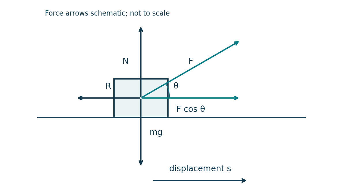
Work is an energy transfer caused by a force acting through a displacement. For a constant force, W = Fs cos θ, where s is the magnitude of the displacement and θ is the angle between force and displacement. Equivalently, multiply the force by the displacement component in its direction. Force is measured in newtons, displacement in metres and work in joules: 1 J = 1 N m. Work is a scalar, even though the force and displacement used to calculate it are vectors.Positive work transfers energy to the chosen object when a force has a component along its displacement. Negative work removes energy from it when the component opposes displacement. A frictional force of constant magnitude R acting over distance s therefore does work −Rs on a sliding object. An exactly perpendicular force does zero work: the normal reaction on a body moving along a level rigid surface does no work. Holding a stationary load also does no mechanical work on that load, despite physiological energy use by the person holding it.Do not substitute total path length without checking the force direction. For each straight part of a journey, identify the displacement and force component along it. For a varying force, the area under a graph of force component against displacement gives work; areas below the axis are negative. A resultant-force graph gives the change in kinetic energy, whereas a graph for one particular force gives only that force’s contribution.
Worked example: an angled pull
A crate travels 8.0 m horizontally under a 45 N pull at 30° above horizontal. Work by the pull is 45 × 8.0 × cos 30° = 312 J, or 3.1 × 10² J to two significant figures. If resistance is 12 N, its work is −96 J. With weight and reaction perpendicular to motion, total work is 216 J, so the crate’s kinetic energy increases by that amount.
A crate moves right. The applied force has horizontal component F cos theta; resistance acts left, weight down and normal force up. Original RevisionTown diagram. Open full-size diagram
Conservation of energy and choosing a system
The total energy of an isolated system remains constant. Energy can move between stores inside that system, but no energy crosses its boundary. For a system that is not isolated, account for energy entering or leaving its boundary; energy is never created or destroyed. Begin an energy calculation by naming the system, its initial and final states, and the transfers across its boundary. A falling object and Earth form a useful combined system: their gravitational potential energy decreases as the object gains kinetic energy. If air resistance matters, some energy also becomes internal energy of the air and object.Mechanical energy means the sum of kinetic and potential energies under consideration. The change in mechanical energy equals the net work done by non-conservative forces in the chosen mechanical model. Mechanical energy is conserved when that net non-conservative work is zero; separate positive and negative transfers can cancel. Total energy is still conserved when mechanical energy decreases. Saying that friction “uses up energy” hides this distinction: friction increases internal energy and may also produce sound.A practical bookkeeping equation is initial energy + energy supplied = final energy + energy transferred out. For a body moving uphill under a motor, the motor’s work may supply both increased gravitational potential energy and increased kinetic energy, as well as energy dissipated against resistance. Do not equate motor work to the increase in one store unless the others are unchanged or negligible.Draw a simple energy-flow diagram before calculating. Check that every energy term has units of joules, that the reference height is used consistently, and that an apparent “missing” term is justified by an assumption. In a laboratory trolley experiment, measured kinetic energy may rise by less than the lost gravitational potential energy because of rolling resistance, pulley rotation and air drag. Such differences test the model rather than disproving energy conservation.
Efficiency and useful output
Efficiency η is useful energy output divided by total energy input for the same process and interval. It is dimensionless and may be written as a fraction or multiplied by 100% to give a percentage. Decide which output is useful for the stated purpose: the heating of a motor is usually unwanted, whereas heating in an electric kettle is the intended output. Efficiency cannot exceed one when the energy inputs and useful outputs of the chosen system have all been counted consistently.For steady operation over a common time interval, η = useful output power / total input power. Rearranging gives useful output = η × input, and required input = useful output / η. Convert a percentage such as 72% to 0.72 before using it as a multiplier. The energy transferred to unwanted stores is input minus useful output; it is not η times the input.For sequential energy-conversion stages, multiply their fractional efficiencies only when the useful output of one is precisely the input of the next. Two stages with efficiencies 0.80 and 0.65 have combined efficiency 0.52. Adding efficiencies or averaging them would not represent the actual flow of energy.
Worked example: lifting water
A pump raises 120 kg of water through 6.0 m at constant speed. With g = 9.81 m s−2, useful energy is mgh = 7063 J. At 64% efficiency the required input is 7063 / 0.64 = 1.10 × 10⁴ J. The remaining 3.97 × 10³ J is transferred to other stores, such as internal energy. If the lift takes 25 s, useful power is 283 W and input power is 441 W.
Power and the derivation of P = Fv
Power is the rate of doing work, or rate of energy transfer. Average power P = W / t for work W done during an elapsed time t. The watt is one joule per second. Power describes how quickly energy is transferred, not how much energy is stored. Two motors can perform the same work but have different powers if they take different times.For a constant force parallel to displacement, work in a short time interval is ΔW = FΔs. Divide by Δt: ΔW / Δt = F(Δs / Δt). As the interval becomes small, Δs / Δt becomes the instantaneous speed v, giving P = Fv. More generally, only the force component along the velocity contributes: P = Fv cos θ. This is the power transferred by the specified force; it need not equal the rate of change of kinetic energy unless that force is the resultant.A vehicle moving in a straight line at constant speed has zero resultant force, but its engine can deliver positive power. The driving force balances resistance, and engine work is transferred to other stores rather than increasing kinetic energy. At a given engine power, the driving force P / v decreases as speed increases. Do not use this relation at v = 0 to claim a real engine produces infinite force; actual engines and transmissions have force and torque limits.To measure average useful lifting power, measure the lifted mass, vertical height and elapsed time, then use mgh / t. Use several repeated lifts and a sufficiently long interval to reduce timing percentage uncertainty. Compare this useful power with separately measured input power when calculating efficiency, and distinguish an average over the lift from power at one instant.
Gravitational potential energy in a uniform field
Gravitational potential energy belongs to the interaction between an object and the gravitational field. In a uniform field, weight mg is constant. Imagine raising mass m slowly through vertical height Δh so that its kinetic energy is unchanged. The upward lifting force balances mg. Work against gravity is force × vertical displacement = mgΔh; this becomes increased gravitational potential energy. Therefore ΔEP = mgΔh.This derivation assumes a uniform gravitational field, so g does not vary appreciably over the height change. Near Earth’s surface this is normally a good approximation for everyday heights. A positive Δh gives increased potential energy; a negative Δh gives a decrease. The zero height is a chosen reference and may be anywhere convenient. Differences in potential energy determine the physical predictions, not the arbitrary numerical value assigned at one point.Only vertical height change matters, not the distance travelled along a slope. Raising a load along a gentle frictionless slope requires a smaller force over a greater distance and gives the same increase mgΔh as a vertical lift. If friction acts, the supplied work is greater than mgΔh. If the load accelerates, some supplied work also increases its kinetic energy.For example, a 3.0 kg object descending by 2.5 m has ΔEP = 3.0 × 9.81 × (−2.5) = −73.6 J. Gravity does +73.6 J of work on it. The equality of these magnitudes does not establish its final speed until other energy transfers and its initial speed have been considered.
Kinetic energy and combined problems
To derive the kinetic energy of a moving mass, consider a constant resultant force F accelerating mass m from speed u to speed v over distance s along a straight line. Newton’s second law gives F = ma, while the constant-acceleration relation gives v2 − u2 = 2as. Thus resultant work Fs = mas = (1/2)m(v2 − u2). Identifying work as the change in kinetic energy, and choosing zero kinetic energy at rest, gives EK = (1/2)mv2.Kinetic energy is non-negative and depends on speed squared. Doubling speed quadruples kinetic energy; reversing the direction without changing speed leaves it unchanged. A change in kinetic energy uses (1/2)m(v2 − u2), not (1/2)m(v − u)2. The derivation uses constant acceleration for simplicity; the energy expression also applies to ordinary non-relativistic translational motion with changing acceleration.
Worked example: descent with resistance
A 0.80 kg trolley starts from rest and loses 0.45 m in vertical height. Resistance transfers 0.72 J to internal energy. Its kinetic energy at the bottom is 0.80 × 9.81 × 0.45 − 0.72 = 2.812 J. Hence v = √(2 × 2.812 / 0.80) = 2.65 m s−1. A frictionless calculation would predict a larger speed.When testing such a prediction, a light gate measures speed over a short distance; its result approximates instantaneous speed only if speed changes little while the flag passes. Check uncertainty before interpreting a small energy mismatch. For a calculated kinetic energy, the percentage uncertainty is approximately the percentage uncertainty in mass plus twice that in speed, using the usual maximum-uncertainty convention.
Check your understanding
A vehicle moving in a straight line at constant speed has zero power output.Its resultant force and kinetic-energy change are zero, but its driving force can do work against resistance at power Fv.Energy dissipated by friction disappears.Mechanical energy is transferred chiefly to internal energy; total energy is conserved.Double speed means double kinetic energy.Kinetic energy depends on speed squared, so it becomes four times as large.The distance travelled up a slope is the height in mgh.Use only the vertical height change; the slope distance belongs in work against a force along the slope.
The PDF contains the full unit practice set. Reveal an answer only after you have committed to a method.
U5-Q1 · 5 marks
A 60 N force pulls a crate 5.0 m horizontally at 40° above horizontal. A constant 18 N resistance acts. (a) Calculate work done by the pulling force. [2] (b) Calculate work done by resistance. [1] (c) State the work done by the normal reaction and find total work on the crate. [2]Show the worked answer to U5-Q1
(a) Only the horizontal force component contributes: W = 60 × 5.0 × cos 40° = 229.8 J ≈ 230 J. (b) WR = −18 × 5.0 = −90 J. (c) The normal reaction is perpendicular to displacement, so its work is zero. Weight also does zero work. Total work = 229.8 − 90 = 139.8 J ≈ 140 J.
U5-Q7 · 6 marks
(a) Use F = ma and v2 = u2 + 2as to derive EK = (1/2)mv2, taking kinetic energy as zero at rest. [3] (b) A 900 kg car speeds up from 10 to 16 m s−1. Find its increase in kinetic energy. [2] (c) Explain the error in using (1/2)m(16 − 10)2. [1]Show the worked answer to U5-Q7
(a) Resultant work W = Fs = mas. From the motion equation, as = (v2 − u2) / 2, so W = (1/2)m(v2 − u2) = ΔEK. With u = 0 and initial kinetic energy zero, EK = (1/2)mv2. (b) ΔEK = (1/2) × 900 × (256 − 100) = 70 200 J. (c) The difference of the squared speeds is required, not the square of their difference; these are algebraically different.
U5-Q12 · 2 marks
Diagnostic multiple choice. A car’s speed increases by 20% while its mass stays constant. By what percentage does its kinetic energy increase? Choose one option and justify it. [2]
A. 20%
B. 40%
C. 44%
D. 144%
Show the worked answer to U5-Q12
Correct option: C. The new energy is (1.20)2 = 1.44 times the original, so the increase is 44%. A treats energy as proportional to speed. B doubles the percentage change as though it were an exact rule for a substantial change; that is only a small-change approximation. D gives the final energy as a percentage of the original, not its percentage increase.
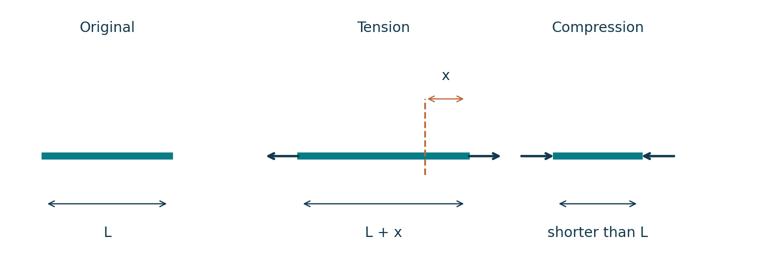
A solid deforms when forces alter its dimensions. In the one-dimensional situations used here, tensile forces pull its ends apart and compressive forces push them towards one another. The forces act along the specimen’s length. Tension may extend a wire or spring; compression may shorten a spring or support. A body can be in equilibrium while deformed: equal opposite end forces give zero resultant force but still produce internal stress.The load is the applied force, measured in newtons. A hanging mass m gives a load approximately mg when stationary; the numerical mass in kilograms is not itself the load. Extension x is final length minus original length, x = L − L0. Compression can be described as the positive decrease in length, L0 − L, when using a magnitude convention. State the convention before applying signed equations.The limit of proportionality is the point beyond which force is no longer directly proportional to extension. On a force–extension graph, the initial straight line through the appropriate zero becomes curved after this point. Direct proportionality means F/x is constant and a doubling of force doubles extension. A graph that is straight but has a non-zero intercept may indicate an initial load, an incorrectly set zero or another offset; check the experimental definition of extension before interpreting it.When investigating a spring, support it securely beside a vertical scale, attach a small pointer, record its unloaded position, and add known loads in small steps. Read at eye level to avoid parallax and allow oscillations to stop. Remove loads gradually and record the return readings as well; the unloading data help determine whether the deformation is reversible.
Tension increases wire length from L to L plus extension x. Compression shortens it. Original RevisionTown diagram. Open full-size diagram
Hooke’s law and spring constant
Within the limit of proportionality, Hooke’s law states that extension is proportional to the applied tensile force. Using magnitudes, F = kx, where k = F/x is the spring constant, or stiffness, in N m−1. The restoring force exerted by the spring acts opposite the deformation; a signed restoring-force equation may therefore be written Frestoring = −kx. Do not insert this minus sign into a magnitude-only energy calculation.For a graph with force on the vertical axis and extension on the horizontal axis, k is the gradient. For a graph of extension against force, the gradient is 1/k. Convert millimetres to metres before reporting stiffness in N m−1; 1 N mm−1 = 1000 N m−1. The value F/x is a constant only while the load–extension relation is proportional.
Worked example: finding stiffness from data
A spring’s extension changes from 12.0 mm to 32.0 mm when load increases from 1.8 N to 4.8 N. Assuming both points lie on the same straight-line region, k = ΔF/Δx = (4.8 − 1.8)/(0.0320 − 0.0120) = 150 N m−1. A load of 3.0 N then gives x = F/k = 0.020 m = 20 mm, provided the spring remains in that region.Use a best-fit line through several measurements rather than relying on one F/x ratio; this reduces sensitivity to a single uncertain reading. A large gradient triangle reduces the percentage uncertainty in the coordinate differences. Inspect residuals or visible curvature rather than forcing a straight line through points beyond proportional behaviour.
Stress, strain and Young modulus
Tensile stress σ is tensile force divided by original cross-sectional area: σ = F/A. Its unit is N m−2, equivalent to the pascal. A smaller cross-sectional area gives greater stress for the same force, explaining why a thin wire may fail under a load safely carried by a thicker wire of the same material. Use the original area in the ordinary small-deformation model considered here.Tensile strain ε is extension divided by original length: ε = x/L. It is a ratio of lengths and has no unit. Strain 0.002 means an extension equal to 0.2% of original length, not 0.002 m. Young modulus E is the ratio of tensile stress to tensile strain in the proportional region: E = σ/ε = FL/(Ax). Its unit is pascals because strain is dimensionless. A larger E means a material requires greater stress to produce a given small strain.Young modulus is a material property within the stated conditions; spring constant describes the stiffness of the particular specimen. Rearranging gives k = F/x = EA/L for a uniform straight wire obeying Hooke’s law. Wires of the same material and length become four times as stiff if their diameters double, because A = πd2/4. A wire twice as long has half the stiffness if material and area stay unchanged.
Worked example: extending a wire
A wire has L = 1.80 m, diameter 0.40 mm and E = 2.0 × 10¹¹ Pa. Its area is π(0.00040)2/4 = 1.257 × 10⁻⁷ m2. Under a 12 N tensile load, x = FL/(AE) = 8.59 × 10⁻⁴ m = 0.86 mm. Stress is 9.55 × 10⁷ Pa and strain is 4.77 × 10⁻⁴.
Measuring Young modulus of a metal wire
Use a long, thin, uniform metal wire fixed securely at its upper end, carrying a load hanger at its lower end. A small preload straightens the wire and removes kinks without approaching its elastic limit. Measure the test length L between the fixed support and the extension marker. Measure wire diameter d with a micrometer at several positions and in two perpendicular orientations, checking its zero first. Use the mean diameter to calculate A = πd2/4.Measure small extensions with a travelling microscope, micrometer arrangement or suitable displacement sensor. Establish a reference reading with the preload present. Add known masses in small equal steps, wait for oscillations to cease and record the change in position relative to that reference. The extra force is ΔF = Δmg; use matching extra extension Δx. Plot added force against extension, fit the straight portion and calculate E = (L/A) × gradient. An extension-against-force plot instead gives E = L/(A × gradient).A nearby reference wire carrying a constant load can help detect movement of the support and common temperature changes; measure the test wire’s extension relative to it. Keep temperature approximately constant, avoid drafts, and prevent the load touching the floor. Repeat measurements during unloading: failure to return to the initial reference indicates that the tested load range may have caused permanent deformation. Use a safety screen or eye protection and a tray close below the masses in case the wire breaks.For a single-reading calculation E = 4FL/(πd2x), approximate maximum fractional uncertainty is ΔE/E = ΔF/F + ΔL/L + 2Δd/d + Δx/x. The diameter contribution is doubled because area depends on d squared. A longer test wire produces a larger measurable extension at the same stress, reducing extension percentage uncertainty. Never increase load past a safe region merely to obtain a larger extension.
Elasticity, plasticity and the limits on a graph
Elastic deformation disappears when the deforming force is removed: the specimen returns to its original dimensions. Plastic deformation leaves a permanent change after unloading. The elastic limit is the largest deformation or corresponding load for which complete recovery is possible. It is a different concept from the limit of proportionality, which concerns the shape of the loading relationship.A material can respond nonlinearly yet still return to its original length. Therefore a curved force–extension graph alone does not prove plastic deformation. To test reversibility, unload and compare the final length with the original. Conversely, Hooke’s law should not be extended to all elastic behaviour; it describes the proportional subset.On a loading and unloading graph, a residual extension at zero force shows permanent deformation. The work supplied while loading is the area beneath the loading curve. The energy returned mechanically during unloading is the area beneath the unloading curve. If the paths differ, the difference between their areas is energy not returned mechanically in that cycle, generally appearing as internal energy and associated irreversible changes. These graphical statements use the same axes and the correct loading direction.In practical data, small differences between initial and final readings may be due to uncertainty, a shifted support, instrument drift or insufficient settling time. Do not claim a plastic change unless the difference is larger than the plausible reading uncertainty and the apparatus is stable. Repeated low-load checks help distinguish apparatus movement from a real material response. Describing a sample as “strong”, “stiff” or “elastic” addresses different properties: resistance to failure, resistance to deformation and ability to recover must not be confused.
Work and elastic potential energy
When a deforming force moves its point of application through a small extension Δx, the work is approximately FΔx. Adding these contributions gives the area beneath the force–extension graph. The horizontal coordinate must be extension or displacement, not strain unless an appropriate conversion is made. A graph area in N mm must be multiplied by 10−3 to obtain joules.In the proportional region the graph from the origin is a straight line, so its area is a triangle. Elastic potential energy stored is EP = (1/2)Fx = (1/2)kx2. The factor one-half occurs because force rises from zero to F while the spring is stretched; using Fx would assume the final force acted throughout. This expression assumes an initially undeformed spring and reversible proportional deformation, with no significant loss.
Worked example: energy stored
A spring with k = 250 N m−1 is extended by 0.040 m. Its final load is 10 N and its energy is (1/2) × 250 × 0.0402 = 0.200 J. Extending it further to 0.060 m raises stored energy to 0.450 J. The extra work is 0.250 J, found by subtracting energies; it is not (1/2)k(0.020)2.For a nonlinear graph, find the actual area using geometric sections or a stated approximation such as trapezia; (1/2)Fx is not automatically valid. For a spring releasing energy into a moving object, equate the decrease in spring energy to the gain in kinetic and other energy stores, including gravitational changes or friction where relevant. Check that a chosen energy-transfer model respects the spring’s permitted deformation range.
Check your understanding
Elastic means obeying Hooke’s law.Elastic means full recovery after unloading. A response can be elastic and nonlinear.Young modulus is measured in N m⁻¹.Young modulus is stress/strain and is measured in Pa. N m⁻¹ is the unit of spring constant.Equal opposite forces cannot stretch a wire.They can deform its ends relative to one another while keeping the whole wire in equilibrium.Stored energy is always final force multiplied by extension.For proportional loading from zero, the average force is half the final force, giving energy ½Fx.
The PDF contains the full unit practice set. Reveal an answer only after you have committed to a method.
U6-Q1 · 5 marks
A straight spring has unloaded length 0.180 m. Opposite tensile forces of 4.0 N act at its ends, giving length 0.205 m. (a) Define load and find the extension. [2] (b) Explain why zero resultant force does not mean zero deformation. [1] (c) Explain how the deformation differs if the end forces are compressive and state what the limit of proportionality identifies. [2]Show the worked answer to U6-Q1
(a) Load is the applied force, here 4.0 N (not the sum 8.0 N of equal opposite end forces). Extension = 0.205 − 0.180 = 0.025 m. (b) The forces act on opposite ends and stretch the spring even while the whole spring is in equilibrium. (c) Compressive forces shorten it along its axis. The limit of proportionality marks the end of the region in which force is directly proportional to deformation.
U6-Q7 · 5 marks
A specimen’s force–extension graph is straight up to 18 N, then curves. If unloaded from 22 N, it returns to its initial length. If unloaded from 27 N, 0.8 mm of extension remains. (a) Identify the limit of proportionality. [1] (b) Explain why 22 N has not exceeded the elastic limit, and give a bounded statement about that limit. [2] (c) Name and explain the deformation remaining after the 27 N test. [2]Show the worked answer to U6-Q7
(a) The limit of proportionality is at 18 N. (b) Full recovery from 22 N means deformation at that load is elastic despite nonlinearity. The elastic-limit load is at least 22 N but below 27 N, assuming the tests describe the same initially unaltered response. (c) The remaining 0.8 mm is plastic, or permanent, deformation: the original length is not recovered after removal of load.
U6-Q12 · 2 marks
Diagnostic multiple choice. A material’s loading graph becomes curved at high load, but on unloading it returns completely to its original length. Which conclusion is supported? Choose one option and explain. [2]
A. Its elastic limit has definitely been exceeded.
B. It shows plastic deformation whenever the graph is curved.
C. It has passed the limit of proportionality but the deformation remains elastic.
D. Its Young modulus must be zero.
Show the worked answer to U6-Q12
Correct option: C. Curvature means force is no longer directly proportional to extension; full recovery means the deformation is elastic. A and B incorrectly identify the proportional limit with the elastic limit or assume nonlinearity proves permanence. D has no basis: a non-proportional graph does not imply zero stiffness or zero Young modulus.
A progressive wave is a travelling disturbance that transfers energy from one region to another. In a rope, a moving hand starts a disturbance and neighbouring rope elements pass it along. In a long spring, either sideways displacements or alternating compressions can travel. A ripple tank shows travelling surface disturbances. For these mechanical examples, matter oscillates about equilibrium positions rather than travelling with the wave over large distances. Energy propagates even though there is no overall transport of the medium in the ideal wave model.Displacement is a particle’s directed distance from its equilibrium position at a specified instant. Amplitude A is the maximum magnitude of displacement. Period T is the time for one complete oscillation, and frequency f is the number of complete oscillations per second: f = 1/T. Frequency is measured in hertz, Hz = s−1. Wavelength λ is the shortest distance between two points in the same phase, such as adjacent crests. Wave speed v is the speed at which a fixed feature of the disturbance travels.Phase specifies the stage of an oscillation. Points in phase have corresponding displacements and directions of motion; points in antiphase differ by 180° or π radians. Along a sinusoidal progressive wave, phase difference magnitude is 360° × Δx/λ, or 2πΔx/λ radians, with complete cycles equivalent. At one position, a time separation Δt gives phase difference 360° × Δt/T.During one period a crest travels one wavelength, so v = distance/time = λ/T. Since f = 1/T, v = fλ. This speed is not the oscillating particle’s speed.
Worked example: ripple measurements
A ripple pattern has wavelength 18 mm and produces 25 crests per second at a point. Its speed is 25 × 0.018 = 0.45 m s−1 and period is 0.040 s. Two points 4.5 mm apart along propagation differ in phase by 360° × 4.5/18 = 90°.
Reading wave graphs and the oscilloscope
A displacement–distance graph is a snapshot of different positions at one time. The separation of adjacent equivalent points gives wavelength, and the largest vertical displacement gives amplitude. A displacement–time graph records one position as time passes; equivalent points give period instead. Check the horizontal axis before choosing an equation: the numerical spacing of peaks has no meaning without its unit.A cathode-ray oscilloscope (CRO) displays an input potential difference on the vertical axis against time on the horizontal axis when its time-base operates. The time-base setting gives time per horizontal division. If one complete cycle occupies N divisions, T = N × time per division and f = 1/T. Measure several cycles and divide their total duration by the number of complete periods to reduce reading uncertainty.The y-gain gives voltage per vertical division. Signal amplitude is the vertical distance from the equilibrium line to a peak multiplied by the y-gain. Peak-to-peak voltage is twice the amplitude for a symmetric sinusoid. A microphone-connected CRO measures electrical signal amplitude; obtaining sound-particle displacement requires a calibration or additional information. Do not label a voltage reading as a physical displacement.
Worked example: CRO settings
A sinusoidal trace spans four complete cycles across 10.0 divisions with time-base 0.20 ms per division. Total time is 2.00 ms, so T = 0.500 ms and f = 2000 Hz. At y-gain 0.50 V per division, a peak-to-peak height of 6.0 divisions gives 3.0 V peak-to-peak and amplitude 1.5 V. Reading across multiple cycles is preferable to measuring the 2.5-division period alone.
Wavelength is a repeat distance on a displacement–distance graph; period is a repeat time on a displacement–time graph. Original RevisionTown diagram. Open full-size diagram
Transverse and longitudinal descriptions
In a transverse wave, the oscillations are perpendicular to the direction of energy propagation. A wave on a stretched rope is a clear example. In a longitudinal wave, the oscillations are parallel to propagation; a sound wave in air consists of moving regions of compression and rarefaction. Compressions have greater density and pressure than the equilibrium medium, while rarefactions have lower density and pressure.For either type, wavelength is the separation between corresponding features: adjacent crests for a transverse sinusoidal sketch, or adjacent compression centres for a longitudinal sketch. The distance from one compression centre to the next rarefaction centre is λ/2, not λ. A longitudinal wave can be drawn as a sinusoidal displacement–distance graph, but the curve is a graph of displacement rather than the shape of a sideways-moving medium.When particle displacement in a longitudinal wave is plotted vertically for convenience, positive displacement must be understood as motion in a chosen direction along the wave, such as rightwards. To find a compression from this displacement graph, consider neighbouring particles: where displacement decreases as equilibrium position increases, neighbours move closer together. A maximum compression is not the point of greatest particle displacement; in a sinusoidal wave it lies at a suitable displacement zero-crossing.Pressure–distance and particle-displacement–distance graphs therefore show the same wavelength but have shifted peaks. Label the plotted quantity carefully. Likewise, the slope of a displacement–time graph gives the particle’s velocity component, whereas its wavelength and frequency determine propagation speed. Neither slope should be casually called “the wave speed”.
Compression centres coincide with negative displacement gradients, not peaks of the displacement graph. Original RevisionTown diagram. Open full-size diagram
Energy transfer, intensity and amplitude
Intensity I is power crossing a surface divided by its area, with the surface taken perpendicular to the direction of energy travel: I = P/A. Its unit is W m−2. If power is not spread uniformly, this simple expression gives an average over the specified area. Intensity refers to energy transferred each second through each unit area, rather than the total energy stored in a wave.For otherwise unchanged progressive waves in the same medium, intensity is proportional to amplitude squared. Thus I2/I1 = (A2/A1)2. Doubling amplitude produces four times the intensity, while reducing intensity to one-quarter leaves half the amplitude. This comparison assumes quantities such as frequency and medium remain fixed; changing unrelated wave properties can change the proportionality constant.For an ideal point source radiating power P uniformly in all directions, the same power crosses each surrounding sphere. Its area is 4πr2, giving I = P/(4πr2). Consequently intensity falls as 1/r2 and amplitude as 1/r, provided absorption, reflections and directional effects are negligible. A narrow beam or strongly reflecting room does not necessarily satisfy this model.For example, a 0.020 W source radiating uniformly has intensity 0.020/(4π × 2.02) = 3.98 × 10⁻⁴ W m−2 at 2.0 m. At 4.0 m the intensity is one-quarter as large and amplitude half as large. In an experiment, subtract detector background, keep its orientation fixed, and check that reflections are not causing local maxima and minima.
The Doppler effect is a difference between emitted and observed frequency caused by relative motion. Here the required model has a sound source moving and an observer stationary relative to the medium. The sound travels through that medium at speed v. The source does not change its emitted frequency fs, but its movement changes the spacing of successive wavefronts along the observer’s direction.One emission period lasts 1/fs. During it, an earlier wavefront travels distance v/fs while the source moves vs/fs. Ahead of an approaching source, the wavefront separation becomes λahead = (v − vs)/fs. The observer receives these fronts at fo = v/λahead = fsv/(v − vs), a higher frequency.Behind a receding source, separation increases, so fo = fsv/(v + vs), a lower frequency. Choose the sign physically before substituting numbers: approaching uses the smaller denominator. The simple formula applies to motion directly towards or directly away from the observer, with source speed below sound speed. At an angle, the relevant line-of-sight geometry must be considered; do not assume the full source speed is directed at the observer.
Worked example: passing sound source
A source emits 680 Hz and moves at 20 m s−1 along the observer’s line, with sound speed 340 m s−1. Approaching frequency is 680 × 340/(340 − 20) = 722.5 Hz. Receding frequency is 680 × 340/(340 + 20) = 642.2 Hz. Sound speed through the stationary air remains 340 m s−1; the observed change arises from wavelength spacing.
A source moving right emits wavefronts closer together ahead and farther apart behind. Observers remain stationary. Original RevisionTown diagram. Open full-size diagram
The electromagnetic spectrum
All electromagnetic waves are transverse and travel at the same speed c in free space, approximately 3.00 × 10⁸ m s−1. They consist of oscillating electric and magnetic fields and need no material medium. Their frequencies and wavelengths differ, linked by c = fλ. In a material medium the propagation speed can be lower and can depend on wavelength; the equal-speed statement here refers specifically to free space.The principal regions, in order of decreasing wavelength and increasing frequency, are radio, microwaves, infrared, visible, ultraviolet, X-rays and gamma rays. The following are useful approximate revision ranges in free space. Region names do not create exact physical boundaries; adjacent conventions can differ, and X-ray and gamma-ray ranges overlap because their production mechanisms also distinguish them.
Region
Approximate wavelength range
Radio
Longer than 10−1 m, extending to many kilometres
Microwaves
10−3 to 10−1 m
Infrared
7 × 10⁻⁷ to 10−3 m
Visible
4 × 10⁻⁷ to 7 × 10⁻⁷ m, or 400–700 nm
Ultraviolet
Approximately 10−8 to 4 × 10⁻⁷ m
X-rays
Approximately 10−13 to 10−8 m
Gamma rays
Typically below 10−10 m; overlaps the short X-ray range
Visible light runs from roughly violet at 400 nm to red at 700 nm. Nanometres convert to metres by multiplying by 10−9. A 600 nm wave has frequency 3.00 × 10⁸/(600 × 10−9) = 5.00 × 10¹⁴ Hz. Violet has a higher frequency than red because its wavelength is shorter, not because it travels faster in vacuum.
Polarisation and successive filters
Plane polarisation restricts transverse oscillations to one direction in the plane perpendicular to propagation. A transverse wave has possible oscillation directions within that plane; a polariser selects one. A longitudinal wave oscillates along its propagation direction and has no corresponding choice of transverse direction, so it cannot show this type of polarisation. Polarisation therefore provides evidence that a wave is transverse.For a plane-polarised electromagnetic wave incident on an ideal polarising filter, Malus’s law is I = I0 cos2 θ. Here I0 is the intensity arriving at that filter, and θ is the angle between the incident electric-field oscillation direction and the filter’s transmission axis. Parallel alignment gives full transmission in the ideal model; perpendicular alignment gives zero. Intermediate angles transmit a nonzero component.After transmission, the wave is polarised along that filter’s axis. For several filters, apply the law at each stage, using the angle between successive relevant directions and the intensity from the preceding stage. Do not apply every filter’s angle relative to the original direction. This syllabus calculation begins with plane-polarised light; no assumption about the transmitted fraction from an unpolarised initial beam is needed.
Worked example: two filters
Plane-polarised light of intensity 80 W m−2 has its electric field at 0°. A first filter is at 30° and a second at 90° to the original direction. After the first, I1 = 80 cos230° = 60 W m−2. The second differs from the new polarisation by 60°, so I2 = 60 cos260° = 15 W m−2. Without the intermediate filter, a single 90° filter would ideally give zero.
Check your understanding
A rope particle travels along the rope at the wave speed.A particle oscillates around equilibrium; the travelling disturbance transfers energy along the rope.A sinusoidal graph must describe a transverse wave.Longitudinal displacement or pressure can also be plotted sinusoidally. Read the axis label and physical displacement direction.An approaching source makes sound travel faster through the air.In this model the wave speed in air is unchanged; the moving source reduces the forward wavefront spacing.Each polariser angle is measured from the original beam direction of polarisation.Use the polarisation direction immediately before that filter, which is set by the previous filter.
The PDF contains the full unit practice set. Reveal an answer only after you have committed to a method.
U7-Q1 · 6 marks
A hand shakes one end of a horizontal rope, producing a sinusoidal progressive wave. Adjacent crests are 0.60 m apart; each point completes 5.0 oscillations per second. (a) Explain what travels along the rope and what the rope particles do. [2] (b) State the wavelength and calculate period. [2] (c) Find the phase difference between positions 0.15 m apart along propagation. [2]Show the worked answer to U7-Q1
(a) A disturbance and energy travel along the rope; its particles oscillate about their equilibrium positions rather than travelling with each crest. (b) λ = 0.60 m. T = 1/f = 1/5.0 = 0.20 s. (c) Phase difference = 360° × 0.15/0.60 = 90°, or π/2 radians.
U7-Q7 · 8 marks
(a) Name all seven principal electromagnetic regions in order of decreasing wavelength and give an approximate wavelength range for each. [4] (b) State the wave type and speed in free space common to all seven. [2] (c) Light has wavelength 450 nm. Calculate its frequency and state whether it is visible. Use c = 3.00 × 10⁸ m s−1. [2]Show the worked answer to U7-Q7
(a) In decreasing wavelength: radio, roughly above 10−1 m; microwaves, 10−3–10−1 m; infrared, 7 × 10⁻⁷–10−3 m; visible, 4 × 10⁻⁷–7 × 10⁻⁷ m; ultraviolet, about 10−8–4 × 10⁻⁷ m; X-rays, about 10−13–10−8 m; gamma rays, typically below 10−10 m. Accept sensible approximate boundary conventions, including X-ray/gamma overlap. Award one mark for correct ordering and three for reasonably complete ranges. (b) All are transverse; all travel at c ≈ 3.00 × 10⁸ m s−1 in free space. (c) f = c/λ = (3.00 × 10⁸)/(450 × 10−9) = 6.67 × 10¹⁴ Hz. It is visible because 450 nm lies between 400 and 700 nm.
U7-Q12 · 2 marks
Diagnostic multiple choice. A source emits frequency fs and approaches a stationary observer at speed 0.10v, where v is sound speed in stationary air. Which expression gives the observed frequency? Choose one option and justify it. [2]
A. 0.90fs
B. 1.10fs
C. fs/0.90
D. fs/1.10
Show the worked answer to U7-Q12
Correct option: C. For an approaching source, fo = fsv/(v − 0.10v) = fs/0.90, approximately 1.111fs. A predicts the wrong direction of change. B uses the simple factor associated with a different observer-motion model, not the required moving-source expression. D uses the denominator for recession.
The principle of superposition states that when waves overlap, the resultant displacement at a point is the algebraic sum of the displacements that each wave would produce separately at that point and instant. Add signed displacements, not intensities. If one wave gives +3 mm and another −2 mm, the result is +1 mm. After overlap, waves continue propagating according to the medium’s behaviour in the linear model.A stationary wave forms when two waves of the same frequency and wavelength, travelling in opposite directions along the same line, superpose. Equal amplitudes give completely stationary nodes. Reflection commonly provides the counter-propagating wave. Some points always cancel and remain at zero displacement: nodes. Midway between neighbouring nodes, reinforcement gives the greatest oscillation amplitude: antinodes. An antinode’s maximum amplitude is twice that of either constituent wave in the ideal equal-amplitude case.A graphical construction plots the two travelling-wave displacement curves at the same time, then adds their vertical coordinates at every position. Repeat at quarter-period intervals. The following example gives resultant displacement at selected positions, with A the amplitude of each travelling wave. It represents successive stationary-wave snapshots, not motion of particles between the columns.
Time
x = 0
x = λ/4
x = λ/2
x = 3λ/4
x = λ
0
0
+2A
0
−2A
0
T/4
0
0
0
0
0
T/2
0
−2A
0
+2A
0
The pattern does not translate. Neighbouring nodes are λ/2 apart; neighbouring antinodes are also λ/2 apart; a node and its nearest antinode are λ/4 apart. All points within one loop oscillate in phase, whereas adjacent loops are in antiphase. Zero displacement at one instant does not identify a node: every point passes through equilibrium, but only nodes remain there. The ideal stationary pattern carries no net energy along the medium because its equal counter-propagating components carry equal opposite energy flows.
Oppositely travelling equal waves superpose. Nodes at zero, half a wavelength and one wavelength stay fixed through the three times shown. Original RevisionTown diagram. Open full-size diagram
Stationary-wave experiments and boundary conditions
For a stretched string, use a vibration generator driven by a variable-frequency signal generator, with the string under tension from a known load over a pulley or an appropriate fixed support. Reflected waves return along the string. Adjust frequency or tension until a clear stable pattern of loops forms. Under the ideal fixed-end approximation, both ends are displacement nodes, so a vibrating length L containing n loops satisfies L = nλ/2. A real driven end may move slightly; identify the effective nodes rather than assuming every support marker is exact.For microwaves, face a transmitter towards a flat metal reflector. Place a movable probe detector in the region of the incident and reflected waves and scan along the propagation direction. Repeated signal minima and maxima indicate nodes and antinodes of the electric-field pattern. Their spacing gives wavelength; the intensity detector’s reading is not a signed field displacement. Keep transmitter frequency, reflector alignment and probe orientation fixed, and avoid strong reflections from other objects. An ideal conducting reflector is an electric-field node at its surface.For an air column, excite a tube with a tuning fork or loudspeaker and vary the air length, for example using an adjustable water level. Resonance is heard as enhanced sound. A rigid closed end is a displacement node and pressure antinode; an open end is approximately a displacement antinode and pressure node. With end corrections neglected, the shortest closed–open resonance has L = λ/4; successive resonant lengths differ by λ/2. A tube open at both ends has displacement antinodes at both ends and its first resonance has L = λ/2.
Worked example: using several spacings
Five consecutive microwave minima span 64.0 mm from first to fifth. There are four gaps, each λ/2, so λ = 2 × 64.0/4 = 32.0 mm. Measuring many gaps reduces fractional position uncertainty. The first-to-fifth distance is not five half-wavelengths: count intervals, not points. If c = 3.00 × 10⁸ m s−1, microwave frequency is 9.38 × 10⁹ Hz.
Diffraction and gap width
Diffraction is the spreading of a wave into regions beyond a gap or around an obstacle, including into a geometrical shadow. It is a wave phenomenon and occurs for water waves, sound, light and other waves. In the same uniform medium, diffraction changes the direction and distribution of the disturbance rather than changing the source frequency or the wavelength set by speed and frequency.In a ripple tank, a straight vibrating bar produces approximately plane wavefronts. Place two barriers across their path with an adjustable gap between them. Illuminate the tank and observe the wavefronts beyond the gap, directly or on a suitable screen. Keep water depth and frequency fixed while changing gap width so that wavelength stays approximately constant. When the gap is many wavelengths wide, most transmitted wavefronts remain almost straight, with spreading near the edges. When gap width is comparable to wavelength, spreading is conspicuous and the emerging fronts become strongly curved.For the same gap, increasing wavelength generally increases diffraction. For the same wavelength, decreasing gap width generally increases the angular spread. A very small gap can transmit little energy even while the transmitted wave is widely spread, so brightness or amplitude alone is not a reliable measure of diffraction. Absorbing tank edges help reduce reflected waves that would obscure the result.The same comparison can be demonstrated with microwaves by scanning a detector behind a variable slit, or with monochromatic light passing through a narrow slit onto a screen. Keep alignment and source settings consistent when comparing patterns. Sound bends noticeably around a doorway because its wavelengths may be comparable with the doorway dimensions; visible-light wavelengths are far smaller than an ordinary doorway, making such spreading much less apparent.
Interference, coherence and demonstrations
Interference is the reinforcement and cancellation pattern formed by superposition of waves. Coherent sources maintain a constant phase difference and have the same frequency. Equal frequency alone is insufficient if their phase relationship changes randomly. For initially in-phase sources, path difference mλ gives constructive interference, while path difference (m + 1/2)λ gives destructive interference, where m is an integer. Unequal amplitudes prevent complete cancellation even at a destructive location.For stable two-source fringes, waves must overlap and remain coherent. For light, use the same polarisation direction or at least components that can interfere; perpendicular polarisations give no ordinary intensity-fringe contrast. Similar amplitudes improve contrast. Narrow sources and suitable geometry help prevent overlapping fringe systems from washing out the pattern. Monochromatic light produces a simple regularly spaced fringe pattern; an extended white source usually requires additional care and can give coloured, overlapping patterns.In a ripple tank, drive two point dippers from one oscillator so that their phase relationship stays fixed. Observe curved lines of strong and weak water motion where their circular waves overlap. Keep water depth constant and reduce reflections at the edges. With sound, feed two loudspeakers from the same signal generator. Move a microphone and sound-level detector along a line across their overlapping beams: repeated loud and quiet positions demonstrate interference. Reflections from walls can obscure the simple two-source pattern.For microwaves, illuminate two slits in a metal screen from one transmitter, then scan a correctly oriented receiving probe beyond them. Record alternating maxima and minima. For light, illuminate two narrow, close slits coherently with a laser or with monochromatic light from a suitable single slit. Observe bright and dark fringes on a distant screen. Never look into a laser or its specular reflections; arrange beams below eye level and use a beam stop. These arrangements share a single source or common oscillator because unrelated emitters generally do not maintain the phase stability required.
Double-slit calculation and measurement
For two narrow slits separated centre-to-centre by a, with a screen distance D much larger than a, a point at small angle θ has path difference approximately a sin θ. For a bright fringe from in-phase illumination, this equals mλ. At small angles, sin θ ≈ tan θ ≈ y/D, so the mth bright fringe lies at ym ≈ mλD/a. Adjacent bright fringes are separated by x = λD/a, giving λ = ax/D.The symbol x is fringe spacing, not the full width of several fringes or the distance to an arbitrary fringe. Adjacent dark fringes have the same spacing; a bright fringe to its neighbouring dark fringe is x/2. The approximation assumes small angles and a distant screen, rather than applying exactly everywhere on an arbitrarily wide pattern. Use the exact geometry if the stated conditions do not justify it.
Worked example: finding wavelength
Double slits have separation 0.25 mm and the screen is 2.00 m away. The distance from the first to the ninth consecutive bright fringe is 38.4 mm, representing eight intervals. Thus x = 38.4/8 = 4.80 mm and λ = (0.25 × 10⁻³)(4.80 × 10⁻³)/2.00 = 6.00 × 10⁻⁷ m = 600 nm.Measure D from the slit plane to the screen and a as centre-to-centre separation. Measuring across many fringes and dividing by the number of intervals reduces the percentage uncertainty in x. Use a darkened background and a fixed reference ruler; avoid moving or tilting the screen between readings. For maximum fractional uncertainty in λ = ax/D, add the fractional uncertainties in a, x and D. Increasing D enlarges fringe spacing but can reduce brightness, so choose a readable pattern rather than the largest possible screen distance.
Double slits are separated by a; screen distance is D; adjacent bright fringe separation is x. Original RevisionTown diagram. Open full-size diagram
Diffraction grating and wavelength experiments
A diffraction grating contains many equally spaced slits or equivalent periodic transmitting regions. Waves from neighbouring slits have path difference d sin θ at angle θ to the normal for normally incident light. A principal maximum occurs when this equals an integer number of wavelengths: d sin θ = nλ. Here d is grating spacing, n = 0, 1, 2, … is the order, and θ is measured from the straight-through central direction. Maxima appear symmetrically on both sides in the ideal arrangement.If a grating has N lines per metre, d = 1/N. A quoted line density per millimetre must first be multiplied by 1000. The allowed orders obey nλ/d ≤ 1 because sin θ cannot exceed one; a calculated larger sine means that order is impossible. A more closely spaced grating sends a given order to a larger angle, but may allow fewer orders.To measure wavelength without requiring a spectrometer, send a narrow monochromatic beam normally through the grating towards a screen at measured distance D. Mark the zero-order spot and the nth-order spots on both sides. If their separation is S, take y = S/2 when the setup is symmetric and calculate θ = arctan(y/D). Then λ = d sin θ/n. Do not replace sin θ by y/D at large diffraction angles. Repeat for several orders or screen distances, keeping the grating normal to the beam, and compare results. Use laser eye-safety precautions.
Worked example: order and wavelength
A grating has 500 lines mm−1, so d = 1/(500 × 1000) = 2.00 × 10⁻⁶ m. First-order light at 17.46° has λ = d sin 17.46° ≈ 6.00 × 10⁻⁷ m. The largest possible integer order is the integer part of d/λ = 3.33, hence n = 3. For uncertainty analysis, larger measured separations usually reduce fractional reading uncertainty, while uncertain normal alignment or misidentified orders can cause systematic error that repetition alone will not remove.
Check your understanding
Add the intensities of coherent waves to find the interference pattern.Add the signed wave displacements or fields first. Intensity then depends on the resultant amplitude squared.Any point at zero displacement is a node.A node stays at zero at all times; other points pass through equilibrium during each oscillation.Two sources of equal frequency are necessarily coherent.Coherence additionally requires a constant phase difference.A node and its nearest antinode are half a wavelength apart.They are λ/4 apart. Adjacent nodes, or adjacent antinodes, are λ/2 apart.The grating angle formula can use slit line density as d.d is spacing in metres, the reciprocal of line density expressed in lines per metre.
The PDF contains the full unit practice set. Reveal an answer only after you have committed to a method.
U8-Q1 · 6 marks
Two equal waves travel in opposite directions along a string. At one point at one instant, their displacements are +4.0 mm and −1.5 mm. (a) State the superposition principle and find resultant displacement. [2] (b) Explain how equal counter-propagating waves form nodes and antinodes. [2] (c) Explain why a point having zero displacement in one photograph is not necessarily a node, and describe how a graphical construction can test for nodes. [2]Show the worked answer to U8-Q1
(a) Resultant displacement is the algebraic sum of the separate displacements: +4.0 − 1.5 = +2.5 mm. (b) At nodes the contributions remain opposite and cancel; at antinodes they reinforce to the greatest oscillation amplitude. Equal-frequency, equal-wavelength, equal-amplitude waves travelling oppositely can give this stationary pattern. (c) Other points pass through equilibrium. Draw both travelling-wave curves at several times and add their signed vertical ordinates; only positions whose resultant remains zero are nodes.
U8-Q7 · 7 marks
A double-slit pattern uses slit separation 0.30 mm and screen distance 1.80 m. The distance from the second to the tenth consecutive bright fringe on one side is 28.8 mm. (a) Find fringe spacing and wavelength. [3] (b) State two approximations needed for λ = ax/D. [2] (c) If uncertainties are 2.0% in a, 1.5% in measured fringe span and 0.5% in D, find maximum percentage uncertainty in λ and explain whether division by eight changes the percentage span uncertainty. [2]Show the worked answer to U8-Q7
(a) There are eight fringe intervals: x = 28.8/8 = 3.60 mm. λ = ax/D = (0.30 × 10⁻³)(3.60 × 10⁻³)/1.80 = 6.00 × 10⁻⁷ m = 600 nm. (b) The screen is far from the slits compared with separation, and observation angles are small, so sin θ ≈ tan θ. (c) Maximum percentage uncertainty = 2.0 + 1.5 + 0.5 = 4.0%. Dividing span and its absolute uncertainty by the exact integer eight leaves fractional uncertainty unchanged.
U8-Q12 · 2 marks
Diagnostic multiple choice. A normally illuminated grating has spacing 1.50 μm and light wavelength 600 nm. How many principal maxima can exist in total, including the central maximum and both sides? Choose one option and justify it. [2]
A. 2
B. 3
C. 5
D. 7
Show the worked answer to U8-Q12
Correct option: C. n ≤ d/λ = 1.50/0.600 = 2.5, so the highest integer order is 2. Orders −2, −1, 0, +1 and +2 give five maxima. A reports only the highest order. B counts orders on one side plus zero but omits the other side. D rounds 2.5 upward to allow a physically impossible third order.
An electric current exists when charge carriers have a net flow through a surface. In a metal, mobile electrons move among a lattice of positive ions; the ions do not travel along the wire. In an electrolyte both positive and negative ions can carry current. Conventional current is defined in the direction in which positive charge would move, so electron drift in a metal is opposite to conventional current. Random electron motion by itself produces no net current.Charge is quantised: it occurs in allowed discrete amounts. An electron carries −e and a proton carries +e, where e = 1.60 × 10⁻¹⁹ C. A doubly charged positive ion carries +2e. For ordinary isolated charged objects, the net charge is an integer multiple of e; the fractional charges of quarks, introduced in Unit 11, are not charges of freely isolated quarks. A charge such as 1.3e is therefore not an allowed charge for an object made by adding or removing whole electrons.Current is charge crossing a section per unit time: I = Q/t for a constant current, so Q = It. One ampere is one coulomb per second. Convert milliseconds to seconds and milliamperes to amperes before substitution. For a varying current the area under an I–t graph gives the charge; the constant-current relation applies to each constant section or to the average current over the interval.
Deriving the drift-current relation
Let a conductor have cross-sectional area A, carrier number density n, mean drift speed v and carrier charge magnitude q. In time t, carriers within a cylinder of length vt cross a section. That cylinder has volume Avt and contains nAvt carriers. Their total charge magnitude is Q = nAvtq. Dividing by t gives I = Anvq. Here n is the number per cubic metre, not the total number or the mass density. A is in m2 and v in m s−1. The expression gives current magnitude; handle the carrier’s sign separately when discussing direction. With several mobile carrier species, add their contributions to conventional current.
Worked example: a fine metal lead
A lead carries 0.48 A for 150 s. Its cross-section is 0.40 mm2 and it has 8.0 × 1028 free electrons per m3. The charge transferred is 0.48 × 150 = 72 C, corresponding to 72/(1.60 × 10−19) = 4.5 × 10²⁰ electrons. Since 0.40 mm2 = 4.0 × 10⁻⁷ m2, v = 0.48/[(4.0 × 10−7)(8.0 × 1028)(1.60 × 10⁻¹⁹)] = 9.4 × 10⁻⁵ m s−1. A slow drift speed is compatible with a large current because the carrier density is enormous.
Conductor volume Avt with fixed positive lattice ions. Electron drift points left, opposite to conventional current. The cylinder contains nAvt carriers. Original RevisionTown diagram. Open full-size diagram
Potential difference, energy and electrical power
The potential difference across a component is the energy transferred from electrical energy to other forms per unit charge passing through it. Thus V = W/Q and W = VQ. One volt is one joule per coulomb. The charge is not consumed: a lamp transfers electrical energy to thermal energy and light while charge continues around the circuit. Identify the energy transfer across the particular component whose voltage is used.Power is the rate of energy transfer. Combining P = W/t, W = VQ and I = Q/t gives P = VI. For a component with resistance R = V/I at its operating point, substitute V = IR to obtain P = I2R, or substitute I = V/R to obtain P = V2/R. These give power in watts when SI units are used. For a nonlinear component such as a hot filament, use the resistance at that operating point, rather than its cold resistance.The direction of a power change depends on what is held fixed. At fixed current, increasing R increases I2R. At fixed voltage, increasing R decreases V2/R because the current falls. Always decide which condition the circuit actually imposes before comparing powers. For constant power, energy transferred over time t is W = Pt; minutes or hours must be converted to seconds if the answer is required in joules.
Worked example: a low-voltage heater
A heater takes 0.80 A from a 12 V supply for 3.0 minutes. Its operating resistance is 12/0.80 = 15 Ω. Its power is 12 × 0.80 = 9.6 W, and its energy transfer is 9.6 × 180 = 1.73 × 10³ J. A cross-check uses Q = 0.80 × 180 = 144 C and W = VQ = 12 × 144 = 1728 J. Both routes describe the same energy, not two separate contributions.
Resistance, Ohm’s law and I–V characteristics
The resistance of a component is the ratio of the potential difference across it to the current through it: R = V/I. The unit is the ohm, Ω, with 1 Ω = 1 V A−1. The rearrangement V = IR is valid using the resistance at that operating point. It does not by itself show that resistance is constant.Ohm’s law states that the current through a conductor is directly proportional to its potential difference, provided its temperature and other physical conditions remain constant. An ohmic conductor therefore has constant R and a straight-line I–V characteristic through the origin. A constant-temperature metallic wire is the standard example. Temperature control is part of the law, not an optional experimental detail.
Reading the three required I–V graphs
With V on the horizontal axis and I on the vertical axis, an ohmic conductor gives a straight line through the origin with positive gradient 1/R. Reversing the voltage reverses the current with the same magnitude.
A filament lamp gives a curve through the origin that becomes less steep as the magnitude of V rises. The negative-voltage branch is the corresponding opposite-sign curve. Higher current heats the filament, increasing the vibrations of the lattice ions. More frequent electron scattering increases resistance. The effect is not that charge is being used up.
A semiconductor diode is strongly asymmetric. In the forward direction, current is initially small and then rises rapidly as the voltage increases. In reverse bias the current is extremely small over the normal operating range. Do not draw a straight-line graph through both quadrants, and do not assume a universal exact switch-on voltage.
At a point on any of these graphs, R = V/I. On an I–V plot, the gradient of the line from the origin to that point is I/V = 1/R. The local tangent gradient of a curved characteristic is not generally 1/R. If the axes are exchanged to V vertically and I horizontally, the straight-line gradient for an ohmic conductor is R. Write the axes before deciding what the gradient means.
Practical method and interpretation
Place the test component, ammeter, protective resistor and variable supply in series; place the voltmeter in parallel with the test component. Begin at low voltage and limit current, especially for a diode. Reverse the supply connections to investigate the opposite polarity, with the power off while rewiring. Record several well-spaced pairs of V and I, repeat readings and plot the curve rather than joining random fluctuations. Keep a wire cool using small currents and brief measurements when testing Ohm’s law; wait for stable temperature when deliberately characterising a lamp. Avoid touching a hot filament or resistor. A systematic curvature is evidence of changing resistance, while scatter alone need not show non-ohmic behaviour.
Three qualitative I–V plots: straight ohmic line, symmetric flattening filament-lamp curve with an origin-to-point chord, and strongly asymmetric diode curve. Original RevisionTown diagram. Open full-size diagram
Resistivity, wire dimensions and uncertainty
For a uniform wire at a stated temperature, R = ρL/A. Resistivity ρ is a material property measured in Ω m; L is the length of the conducting path and A is its cross-sectional area. Doubling L with A unchanged doubles the resistance. Doubling a circular wire’s diameter makes A four times larger and R four times smaller. Resistivity is not generally temperature-independent.A circular wire has A = πd2/4, so ρ = Rπd2/(4L). Convert diameter to metres before squaring. A diameter of 0.30 mm is 3.0 × 10⁻⁴ m, not an area of 0.30 mm2. Use the measured conducting diameter rather than the outside of an insulating coating.
Worked example: finding a material property
A wire of length 1.50 m and diameter 0.320 mm has resistance 0.310 Ω. Its area is π(0.320 × 10⁻³)2/4 = 8.04 × 10⁻⁸ m2. Hence ρ = (0.310)(8.04 × 10⁻⁸)/1.50 = 1.66 × 10⁻⁸ Ω m. The small result is plausible for a good conductor.To measure ρ reliably, use a micrometer at several positions and orientations, check its zero, and average the diameter readings. Measure L between the voltage contacts. Determine R from several V and I readings at low power to limit heating. Alternatively, measure R for several L values: the gradient of an R–L graph is ρ/A. A nonzero intercept may indicate contact or lead resistance, which is separated from the gradient in this method. Include error bars and compare sensible maximum and minimum gradients where required.For an estimated maximum fractional uncertainty, add fractional contributions: Δρ/ρ ≈ ΔR/R + 2Δd/d + ΔL/L. If R is calculated as V/I, ΔR/R ≈ ΔV/V + ΔI/I. The squared diameter makes its fractional uncertainty especially influential. Repeats reduce random scatter; they do not automatically remove a micrometer zero error or a temperature bias. Quote the final uncertainty and round the result consistently.
LDRs and negative-temperature-coefficient thermistors
A light-dependent resistor has high resistance in dim conditions and lower resistance under stronger illumination. Light supplies energy that enables more mobile charge carriers to contribute to conduction in the semiconductor. The resistance change is generally nonlinear, so use supplied data or a calibration curve rather than assuming that doubling the light intensity halves R.The thermistors used in this course have a negative temperature coefficient: their resistance falls when their temperature rises. In their semiconductor material, heating increases the availability of mobile carriers; over the relevant range this effect outweighs increased scattering. This is different from a metal wire, whose resistance normally rises on heating. State the type of component rather than giving a blanket rule that heating always increases resistance.To investigate an LDR, keep lamp position and angle controlled, shield unwanted room light and allow readings to settle. A lamp can also heat the LDR, so minimise that effect. For a thermistor, use a gently stirred water bath and a thermometer close to the sensor, wait for thermal equilibrium, keep connections dry, and use low measuring current to avoid self-heating. Follow the teacher’s electrical and hot-water safety instructions. Record a calibration table of R against the controlled variable and plot a smooth trend.A changing resistance becomes an easily measured changing voltage when the sensor forms one arm of a potential divider. Whether that output rises or falls depends on which component the output is measured across. Unit 10 derives this connection; a sensor’s resistance trend alone does not determine the sign of the output change.
LDR resistance falls nonlinearly as light intensity rises; NTC thermistor resistance falls nonlinearly as temperature rises. Original RevisionTown diagram. Open full-size diagram
Check your understanding
Does a lamp use up current?No. Charge is conserved. A lamp transfers energy from the charges, so the energy per unit charge changes while the series current remains the same.Does V = IR prove that every component obeys Ohm’s law?No. R = V/I defines resistance at an operating point. Ohm’s law additionally requires proportionality and constant resistance under unchanged physical conditions.Is the tangent gradient of an I–V curve always 1/R?No. R = V/I uses the origin-to-point ratio. Only for a straight line through the origin does its tangent gradient equal I/V.Does twice the wire diameter mean half the resistance?No. At the same length and resistivity the area is four times larger, so the resistance is one quarter.Does heating always increase resistance?No. A metal normally increases in resistance, but the NTC thermistors in this syllabus decrease.
The PDF contains the full unit practice set. Reveal an answer only after you have committed to a method.
U9-Q1 · 6 marks
A metal lead carries a steady conventional current of 0.32 A from P to Q for 75 s. (a) Identify the mobile charge carriers and their drift direction. (b) Find the charge crossing a section and the number of electrons involved, using e = 1.60 × 10⁻¹⁹ C. (c) Explain why removing electrons cannot leave an otherwise neutral object with charge +4.0 × 10⁻¹⁹ C.Show the worked answer to U9-Q1
(a) Electrons carry the current and drift from Q to P, opposite to conventional current [2]. (b) Q = It = 0.32 × 75 = 24 C [1]. N = Q/e = 24/(1.60 × 10−19) = 1.5 × 10²⁰ electrons [1]. (c) The proposed charge is 2.5e [1], which would require removing half an electron in addition to whole electrons. Net charge from adding or removing electrons is an integer multiple of e [1].
U9-Q7 · 7 marks
A uniform wire is 2.40 m long and 0.400 mm in diameter. Its measured resistance is 4.20 Ω. (a) Find its resistivity. (b) Find the resistance of a 1.20 m length of the same material at the same temperature with diameter 0.800 mm. (c) For the original wire, the percentage uncertainties in R, L and d are 2.0%, 0.5% and 1.0%. Estimate the maximum percentage uncertainty in ρ and give an absolute uncertainty.Show the worked answer to U9-Q7
(a) A = π(4.00 × 10⁻⁴)2/4 = 1.2566 × 10⁻⁷ m2 [1]. ρ = RA/L = 4.20 × 1.2566 × 10−7/2.40 = 2.20 × 10⁻⁷ Ω m [2]. (b) The length is halved and area quadrupled, so R = 4.20/8 = 0.525 Ω [2]. (c) Maximum percentage uncertainty = 2.0 + 0.5 + 2(1.0) = 4.5% [1]. Absolute uncertainty = 0.045 × 2.20 × 10−7 = 0.10 × 10⁻⁷ Ω m; report approximately (2.20 ± 0.10) × 10−7 Ω m [1].
U9-Q12 · 3 marks
Diagnostic multiple choice. A filament lamp’s I–V graph, with I vertical, becomes less steep at higher positive voltages. Which explanation is best? A: Electrons are used up in the filament. B: The hotter lattice causes greater electron scattering, raising resistance. C: The lamp must obey Ohm’s law because R = V/I can be calculated. D: The filament’s resistance equals the local I–V tangent gradient. Choose one option and reject the others.Show the worked answer to U9-Q12
B is correct [1]. Heating increases scattering and V/I, so the I–V curve flattens [1]. A violates charge conservation. C confuses the definition of resistance with constant resistance under Ohm’s law. D has the wrong ratio and uses a tangent instead of the origin-to-point relation for a nonlinear graph [1 for identifying the three errors].
A circuit diagram describes electrical connections, not the physical placement of equipment. All points joined by an ideal wire belong to one node. A dot marks a junction where conductors connect; crossing lines without a connection mark are not automatically a junction. Components are in series only when the same current must pass through them without a branch between. Components are in parallel only when both ends connect to the same two nodes.Read a circuit by identifying the source terminals, labelling junctions, and tracing each complete conducting path. An ammeter measures branch current and is placed in series; its ideal resistance is zero. A voltmeter measures a potential difference and connects across two points in parallel; its ideal resistance is infinite. A real meter can alter the circuit, so choose suitable ranges and account for loading if specified. Never connect an ammeter directly across a source.
All 27 symbols in the syllabus guide
The accompanying original symbol chart should be used for drawing practice. These identifying features help distinguish similar symbols; use complete connecting leads when drawing a working circuit.
Component
How to recognise it and what it represents
Cell
One long and one short parallel line. The long line marks the positive terminal.
Battery of cells
Repeated long–short pairs; a dashed middle can abbreviate further cells.
Power supply
Two open-circle terminals, with supply type or polarity labelled as needed.
A.C. power supply
Two terminals with a sine-wave mark between them.
Junction of conductors
Joining wires with a filled dot at their meeting point.
Lamp
A circle with a diagonal cross.
Fixed resistor
A rectangle in the conducting path.
Variable resistor
A resistor rectangle crossed diagonally by an arrow.
Thermistor
A resistor crossed by a slanted line with a short bent end, without an arrowhead.
LDR
A resistor with two light arrows pointing towards it.
Heater
A rectangle subdivided by several transverse lines.
Switch
A break with a hinged sloping contact, drawn open or closed.
Earth
A connection to three horizontal bars of decreasing width.
Electric bell
An upward-domed bell outline with two leads beneath.
Buzzer
A downward-curving bowl outline with two leads beneath.
Microphone
A small circle beside a short straight plate, with two leads on the other side.
Loudspeaker
A small rectangular block opening into a flared cone outline.
Motor
A circle containing M; the guide includes a short line under M.
Generator
A box containing G, supplying electrical energy.
Ammeter
A circle containing A.
Voltmeter
A circle containing V.
Galvanometer
A circle with a pointer; a sensitive indicator of small current and its direction.
Potentiometer
A resistor rectangle with a third, arrow-tipped sliding contact touching it.
Oscilloscope
A circle with a small trace-like stepped/sloping line.
Diode
A triangular outline meeting a perpendicular bar; the bar marks the cathode.
LED
A diode with two light arrows pointing away from it.
Capacitor
Two equal parallel plates separated by a gap.
Recognising a symbol does not mean that all of that component’s detailed theory belongs in the AS course. In particular, do not confuse an equal-plate capacitor with an unequal-plate cell, an LDR’s inward light arrows with an LED’s outward arrows, or a two-terminal variable resistor with the three-terminal use of a potentiometer.
E.m.f., terminal potential difference and internal resistance
The electromotive force E of a source is the energy it transfers from another form into electrical energy per unit charge driven around the complete circuit. E = Wsource/Q, measured in volts. A battery converts chemical energy; a generator converts mechanical energy. Despite its name, e.m.f. is not a force in newtons.A potential difference across a load describes energy transferred from electrical energy per unit charge in that part of the circuit. E.m.f. describes the source’s energy supply per charge. They can have the same numerical value for an ideal source, but refer to different energy transfers. For a real delivering source, some electrical energy is dissipated internally before it reaches the external load.Model a source as an ideal e.m.f. E in series with an internal resistance r. With external resistance R, the same current flows through r and R. Energy conservation gives E = IR + Ir, so I = E/(R + r). The terminal p.d., also the external-load p.d., is V = IR = E − Ir. The quantity Ir is the internal voltage drop, often called lost volts; energy is converted to thermal energy internally rather than destroyed. On open circuit I is approximately zero and V approximately equals E. As the load resistance falls, current rises and terminal voltage falls. The model predicts I = E/r for a short circuit, which can be dangerously large: never deliberately short a cell.
Worked example: a real source
A source has E = 9.0 V, r = 1.5 Ω and an external 4.5 Ω resistor. I = 9.0/(4.5 + 1.5) = 1.5 A. The terminal voltage is 9.0 − 1.5(1.5) = 6.75 V. The source supplies EI = 13.5 W; the external resistor receives I2R = 10.125 W and the internal resistor dissipates I2r = 3.375 W. These two powers sum to 13.5 W. Round only at the final stage.To estimate E and r, vary an external load and measure the source terminal V and series I. A graph of V vertically against I horizontally follows V = E − rI: the intercept is E and the negative gradient is −r. Use a current limit, avoid heating and recharge/discharge changes, and take readings promptly. The constant-r model has a limited operating range; curved data may indicate temperature or source-condition changes.
Ideal e.m.f. E and internal resistor r inside a dashed source boundary, with ammeter and external R in the main loop. An ideal voltmeter spans the source terminals. The V–I graph has intercept E and gradient −r. Original RevisionTown diagram. Open full-size diagram
Kirchhoff’s laws and combined resistance
Kirchhoff’s first law states that the total current entering a junction equals the total current leaving it. It follows from charge conservation: charge does not steadily accumulate at a junction in a steady circuit. Assign current directions before writing an equation. A negative solution means the actual current runs opposite to the arrow chosen; it is not an impossible current.Kirchhoff’s second law states that the algebraic sum of potential changes around a closed loop is zero. Equivalently, total e.m.f. around a loop equals total resistive voltage drop when signs are consistent. It follows from energy conservation: a charge returning to its starting point cannot gain net energy merely by completing the loop. Across a source from negative to positive count +E; through a resistor in the assumed current direction count −IR. Traversing a resistor against its current gives +IR. Do not automatically add sources that oppose one another.
Series derivation
At each unbranched connection the first law gives the same current I. Around a loop, V = V1 + V2 + … . Substitute V = IReq and Vi = IRi. Then IReq = IR1 + IR2 + …, so Req = R1 + R2 + … . Series resistance is larger than any one positive resistance because there is one longer resistive path.
Parallel derivation
Each branch joins the same two nodes. Kirchhoff’s second law gives the same V across every branch. The first law gives I = I1 + I2 + … . Using I = V/R gives V/Req = V/R1 + V/R2 + … . Dividing by V gives 1/Req = 1/R1 + 1/R2 + … . For two resistors, Req = R1R2/(R1 + R2). Parallel resistance is smaller than the smallest branch resistance because extra conducting paths are available.
Worked example: a mixed network
An ideal 12 V source feeds a 3.0 Ω resistor in series with a parallel pair of 6.0 Ω and 3.0 Ω. The parallel resistance is (6 × 3)/(6 + 3) = 2.0 Ω, so total resistance is 5.0 Ω and source current is 2.4 A. The series resistor drops 2.4 × 3 = 7.2 V. Both parallel resistors have 12 − 7.2 = 4.8 V across them. Their currents are 0.80 A and 1.60 A, summing to 2.40 A. Checking both the junction current sum and the loop voltage sum catches many errors.For a circuit that cannot be reduced immediately, label nodes and branch currents, write enough independent junction and loop equations, solve them together, then check the signs and total power. A resistor cannot be classified as series or parallel merely because it looks horizontal or vertical on the page.
Potential dividers, sensors and loading
A potential divider uses series resistances to divide a supply voltage. Let Rupper connect the positive supply Vs to junction J, and Rlower connect J to the 0 V rail. With no significant output current, I = Vs/(Rupper + Rlower). The output measured from J to 0 V is the p.d. across the lower resistor: Vout = IRlower = VsRlower/(Rupper + Rlower). The two voltage drops add to Vs. A sliding contact on a uniform resistor varies the fraction of resistance below it and hence the output.For sensor questions always name the output terminals. If the lower component is an LDR, brighter light lowers Rlower and lowers Vout. If the LDR is the upper component, brighter light lowers Rupper and raises Vout. An NTC thermistor follows the same pair of trends on heating: output across the thermistor falls, whereas output across a fixed lower resistor rises when the thermistor is above it. Explain with the divider ratio rather than saying that voltage always follows resistance everywhere.
Worked example: a warming sensor
A 5.0 V divider has a thermistor above J and a 10 kΩ fixed resistor below J. The output is J relative to the lower 0 V rail. When the thermistor is 15 kΩ, Vout = 5.0(10)/(15 + 10) = 2.0 V. When it warms and falls to 5.0 kΩ, Vout = 5.0(10)/(5.0 + 10) = 3.33 V. The current increases, so the p.d. across the unchanged lower resistor increases. If the output were measured across the thermistor instead, it would fall from 3.0 V to 1.67 V.The simple formula assumes the output is unloaded, or connected to an instrument of very high resistance. A finite load connected between J and 0 V lies in parallel with Rlower. First replace that pair by its equivalent resistance, then use the divider formula. For example, with 6.0 V, an upper 2.0 kΩ resistor and lower 4.0 kΩ resistor, the unloaded output is 4.0 V. Adding a 4.0 kΩ load makes the lower equivalent 2.0 kΩ, reducing output to 3.0 V. This is why an ammeter across a divider output is not an acceptable voltage measurement.
Two unloaded 6-volt potential dividers: a lower LDR makes output fall with increasing light, while an upper LDR makes output rise. In both circuits output is junction J relative to 0 volts. Original RevisionTown diagram. Open full-size diagram
Potentiometer comparison and the null method
A comparison potentiometer uses a uniform resistance wire AB carrying a steady current from a separate driver supply. Let A be the high-potential end. If the wire’s material, area and temperature are uniform, resistance and voltage drop are proportional to length: VAJ = kl, where l is distance AJ and k is the potential gradient in V m−1. Keep the driver current fixed between comparisons. This measurement method should not be confused with merely reading a loaded three-terminal variable resistor.To compare a test cell, connect its positive terminal to A and its negative terminal through a sensitive galvanometer to sliding contact J. The test e.m.f. opposes the wire drop. Move J until the galvanometer reads zero. Then the galvanometer branch carries no current, the two connected points have equal potential, and Etest = kl. At balance the test cell supplies no current, so there is no internal drop within it and the method measures its e.m.f. A voltmeter generally draws some current; the null method avoids this loading at balance.The galvanometer’s purpose is to detect zero current and its direction, not to give a voltage reading. A change in deflection direction as the contact passes through balance helps locate the null. Use a protective resistance and brief contact while searching, then increase sensitivity near balance. The main wire current continues to flow at null; only the test branch is current-free.
Worked example: comparing two cells
A reference cell of e.m.f. 1.80 V balances at 0.720 m. The unchanged wire current gives k = 1.80/0.720 = 2.50 V m−1. An unknown cell balances at 0.536 m, so its e.m.f. is 2.50 × 0.536 = 1.34 V. Equivalently Eunknown/Ereference = lunknown/lreference. The ratio of lengths works only if the potential gradient is unchanged.To compare two existing potential differences rather than cell e.m.f.s, connect each pair of points with the appropriate polarity to the null branch in turn. At balance its p.d. equals kl, provided its original circuit conditions are maintained. Balance cannot be found if the required p.d. exceeds the total wire drop, the polarity assists rather than opposes that drop, or a poor connection prevents a meaningful reading. A zero reading caused by an open circuit is not proof of balance: check opposite deflections on either side.Measure balance lengths from the same origin, avoid parallax and press the contact lightly. Long balance lengths reduce the fractional effect of a fixed length-reading uncertainty. If two lengths have independent quoted maximum uncertainties, the maximum fractional uncertainty in their ratio is approximately the sum of their fractional uncertainties. Driver drift and nonuniform wire are systematic problems that repeated length readings alone do not remove.
Separate driver and test-cell branches of a comparison potentiometer. A is the high-potential end of uniform wire AB. Test-cell positive joins A and its negative connects through a galvanometer and protective resistor to slider J. Only the test branch has zero current at balance. Original RevisionTown diagram. Open full-size diagram
Check your understanding
Is e.m.f. a force or the voltage always measured at a battery’s terminals?It is energy supplied per charge, measured in volts. When a real battery supplies current, terminal voltage is lower by Ir.Are two nearby components automatically in series?No. Series means they must carry the same branch current; parallel means they share both end nodes.Does a negative calculated branch current make the circuit impossible?No. It means the current flows opposite to the chosen reference arrow.Does zero galvanometer current mean no current flows anywhere in a potentiometer?No. Only the comparison branch is current-free at balance; driver current continues along the wire.Does a hotter NTC thermistor always make the divider output fall?No. It falls if measured across the thermistor, but rises across the fixed lower resistor when the thermistor forms the upper arm.
The PDF contains the full unit practice set. Reveal an answer only after you have committed to a method.
U10-Q1 · 27 marks
Symbol fluency. Without looking at the chart, draw and label one standard symbol for each item: cell; battery of cells; power supply; a.c. power supply; junction of conductors; lamp; fixed resistor; variable resistor; thermistor; LDR; heater; switch; earth; electric bell; buzzer; microphone; loudspeaker; motor; generator; ammeter; voltmeter; galvanometer; potentiometer; oscilloscope; diode; LED; capacitor. Include leads and preserve the features distinguishing similar symbols.Show the worked answer to U10-Q1
Award one mark for each correctly recognisable labelled symbol, checking against the original symbol chart [27 total]. Essential distinctions: the cell has unequal plates but the capacitor equal plates; the battery repeats cell pairs; a.c. supply includes a wave mark; a junction has a dot; lamp has a cross; fixed resistor is rectangular; variable resistor has a diagonal arrow; thermistor has a bent diagonal line without an arrowhead; LDR arrows point inwards; LED arrows outwards; potentiometer has a separate sliding-contact lead. The heater is subdivided, switch has a movable contact, earth has diminishing bars, bell domes upwards and buzzer bowls downwards. Microphone and loudspeaker have their input/output outlines; M, G, A and V identify their devices; galvanometer has a pointer; oscilloscope a trace; diode has its cathode bar. The chart gives complete shapes and leads.
Answer-key symbol plate 1 of 3: Cell, Battery of cells, Power supply, A.C. power supply, Junction of conductors, Lamp, Fixed resistor, Variable resistor, Thermistor. Original RevisionTown diagram. Open full-size diagram
Answer-key symbol plate 2 of 3: Light-dependent resistor, Heater, Switch, Earth, Electric bell, Buzzer, Microphone, Loudspeaker, Motor. Original RevisionTown diagram. Open full-size diagram
Answer-key symbol plate 3 of 3: Generator, Ammeter, Voltmeter, Galvanometer, Potentiometer, Oscilloscope, Diode, Light-emitting diode, Capacitor. Original RevisionTown diagram. Open full-size diagram
U10-Q8 · 8 marks
Nodes A and B are joined by three separate branches. Branch 1 contains an ideal 9.0 V cell, with its positive terminal at A, followed by a 3.0 Ω resistor leading to B. Branch 2 contains an ideal 3.0 V cell, also with its positive terminal at A, followed by a 6.0 Ω resistor leading to B. Branch 3 is a single 6.0 Ω resistor directly from A to B. Let V = VA − VB, and initially define all three currents from A to B. Find V and the three signed currents, stating each actual direction.
Three parallel branches between top node A and bottom node B. Branch one has a 9.0-volt cell positive toward A and a 3.0-ohm resistor. Branch two has a 3.0-volt cell positive toward A and a 6.0-ohm resistor. Branch three has a 6.0-ohm resistor. All assumed current arrows point A to B. Original RevisionTown diagram. Open full-size diagramShow the worked answer to U10-Q8
For the specified A-to-B traversal, V = 9.0 + 3.0I1, V = 3.0 + 6.0I2, and V = 6.0I3 [3]. The junction equation is I1 + I2 + I3 = 0 [1]. Hence (V − 9)/3 + (V − 3)/6 + V/6 = 0. Multiplying by 6 gives 4V − 21 = 0, so V = 5.25 V [1]. I1 = −1.25 A, meaning B to A; I2 = +0.375 A and I3 = +0.875 A, both A to B [3]. The entering current 1.25 A equals 0.375 + 0.875 A, checking charge conservation.
U10-Q14 · 3 marks
Diagnostic multiple choice. An NTC thermistor connects from the positive rail to J; a fixed resistor connects from J to 0 V. Output is J relative to 0 V. Which statement is correct? A: Warming lowers the output because all warm components have greater resistance. B: Warming raises the output because the upper resistance falls. C: At a potentiometer null, all current in the driver wire stops. D: A galvanometer is connected across a source as an ordinary low-resistance voltmeter. Choose one and explain the errors in the alternatives.Show the worked answer to U10-Q14
B is correct [1]: Vout = VsRfixed/(RNTC + Rfixed) increases as RNTC falls [1]. A misstates the NTC trend. C confuses the zero-current test branch with the still-powered main wire. D confuses current detection with voltage measurement and could cause excessive current [1 for the alternative errors].
In the α-particle scattering experiment, a narrow beam of positively charged α-particles is directed at a very thin metal foil, and a detector records particles emerging at different angles. Most pass approximately straight through; a small fraction undergo large deflections, including a very small number that return towards the incident side. An explanation must account for the rare large deflections as well as the common straight paths.Most particles passing through with little deflection implies that the region producing strong scattering occupies only a tiny part of an atom. Rare, large-angle deflections show that positive charge and substantial mass are concentrated in a very small, dense nucleus. A close approach to that positive region produces strong electrostatic repulsion of the positive α-particle. A spread-out distribution of positive charge would not generate the strong local repulsion needed for the observed large deflections. The nucleus is small compared with the atom, and most of the atomic volume contains no massive nucleus. It is more precise to say this than to imagine that the whole atom is literally devoid of electrons or fields.The simple nuclear model has positively charged protons and electrically neutral neutrons within the nucleus, with negatively charged electrons occupying the surrounding atomic region. A proton has charge +e and mass approximately 1 u; a neutron has charge zero and mass approximately 1 u; an electron has charge −e and a much smaller mass, about 1/1836 of a proton’s mass. Almost all atomic mass is therefore nuclear. In a neutral atom the number of electrons equals the number of protons. The school-level picture of orbital electrons locates them outside the nucleus; a scattering result does not determine detailed electron paths.Typical nuclear and atomic sizes differ by several orders of magnitude: a nucleus is on a scale of femtometres, while an atom is on a scale of 10−10 m. Exact sizes vary with the element and are not inferred from the fraction scattered alone without a more detailed model. The qualitative conclusion required here is a nucleus occupying a very small fraction of atomic volume.
Alpha-particle paths around a tiny positive nucleus within a much larger faint atomic boundary. Different particles undergo differing deflections, including one that returns towards the incident side. No path intersects the nucleus. Not to scale. Original RevisionTown diagram. Open full-size diagram
Nuclides, isotopes and the atomic mass unit
The proton number Z counts protons in a nucleus and determines the element. The nucleon number A counts all protons and neutrons, so neutron number N = A − Z. A and Z are whole-number counts and have no units. Represent a nuclide as AZX, with the nucleon number at the upper left and proton number at the lower left of the chemical symbol. An ion’s net charge, if needed, is written separately at the upper right; it is not Z.Isotopes are nuclei of the same element with the same proton number and different neutron numbers. They therefore have different A. Their neutral atoms contain the same number of electrons, although their nuclear masses and stability can differ. Removing an electron makes an ion, not a new isotope. Do not subtract electron number when finding neutron number.
Worked example: isotope and ion bookkeeping
The ion 3717Cl− has 17 protons and 37 − 17 = 20 neutrons. Its negative unit charge means it has one electron more than protons, so it contains 18 electrons. The neutral isotope 3517Cl instead has 18 neutrons and 17 electrons. The nuclei have the same proton number and belong to the same element; their different neutron counts make them isotopes.The unified atomic mass unit u is one twelfth of the mass of a neutral carbon-12 atom at rest in its ground state. Use 1 u ≈ 1.66 × 10⁻²⁷ kg. It is a mass unit, not a charge unit and not the nucleon count A. A nucleus with A nucleons has mass approximately A u, but precise measured masses are not exactly equal to that integer because proton and neutron masses and binding effects matter. Keep a distinction between a neutral atomic mass and a nuclear mass if a question specifies which is supplied.
Worked example: changing mass units
A specified atom has measured mass 19.99 u. Its mass in kilograms is 19.99 × 1.66 × 10−27 = 3.32 × 10⁻²⁶ kg. Conversely, a particle of mass 6.64 × 10⁻²⁷ kg has mass (6.64 × 10⁻²⁷)/(1.66 × 10−27) = 4.00 u. Multiplication converts u to kg; division converts kg to u.
Radiations, antiparticles and neutrinos
Nuclear radiation is emitted during changes in a nucleus. An α-particle is a helium nucleus containing two protons and two neutrons. Its nucleon number is 4, charge is +2e, and mass is approximately 4 u or 6.64 × 10⁻²⁷ kg. It is not a neutral helium atom because it has no accompanying orbital electrons.β− radiation consists of electrons created in the nuclear transformation; these are not orbital electrons simply knocked out of the atom. Each has charge −e and rest mass 9.11 × 10⁻³¹ kg, about 5.49 × 10⁻⁴ u. β+ radiation consists of positrons, with charge +e and the same rest mass as electrons. Neither electron nor positron is a nucleon, so each is assigned A = 0 in a nuclear equation.γ radiation consists of high-energy electromagnetic photons. A photon has zero electric charge and zero rest mass, but carries energy and momentum. Gamma emission by an excited nucleus changes its energy state without changing A or Z. Zero rest mass does not mean zero energy.An antiparticle has the same rest mass as its corresponding particle and opposite electric charge. Thus the positron is the electron’s antiparticle, not a proton: a proton is far heavier. For neutral particles the opposite of zero charge is still zero; the particle and antiparticle are distinguished by other particle properties. No detailed treatment of those additional properties is required here.In β− decay an electron antineutrino is also emitted; in β+ decay an electron neutrino is emitted. Use νe for an electron neutrino and ν̅e for an electron antineutrino. Both carry zero electric charge and no nucleon number. They are extremely light; no numerical neutrino mass is required. They carry away a variable share of the released energy, which is crucial to explaining the beta energy spectrum.Compare properties separately: mass, charge and physical composition answer different questions. A γ photon and a neutron are both electrically neutral but are not the same kind of particle and do not have the same rest mass. A positron and a proton both carry +e but again have very different masses and internal structure.
Decay equations, conservation and energy spectra
In a nuclear process, conserve the total nucleon number and total electric charge. In the notation used for decay equations, add the upper numbers on each side and independently add the lower charge numbers. The lower number on an emitted electron is −1; it is not a count of negative protons. Neutrinos contribute zero to both totals. Conserving charge is not the same as keeping the daughter nucleus’s proton number unchanged.
Alpha decay
An α-particle removes two protons and two neutrons. Therefore the daughter has nucleon number A − 4 and proton number Z − 2. For example, 22688Ra → 22286Rn + 42He. The upper totals are 226 = 222 + 4 and the lower totals 88 = 86 + 2. The daughter is a different element.
Beta-minus and beta-plus decay
In β− decay, a neutron in the nucleus changes into a proton, emitting an electron and an electron antineutrino: n → p + e− + ν̅e. A is unchanged and the daughter Z increases by one. A complete nuclear example is 2712Mg → 2713Al + 0−1e + ν̅e. Charge checks as 12 = 13 − 1; nucleon count remains 27.In β+ decay, within an energetically allowed nuclear transformation, a proton changes into a neutron while a positron and electron neutrino are emitted: p → n + e+ + νe. A stays the same and daughter Z decreases by one. For example, 189F → 188O + 0+1e + νe. The lower totals are 9 = 8 + 1. This equation does not claim that an isolated free proton spontaneously decays this way.
Why alpha energies are discrete but beta energies spread out
Nuclear energy states are discrete. For an alpha transition to a particular daughter state, the available energy and two-body recoil determine a particular α energy. Several allowed daughter states can produce several separate α lines, rather than a continuous band. In beta decay the electron or positron shares the available energy with the (anti)neutrino and the recoiling daughter. Different decays can divide the energy differently, so beta particles have a continuous range from low energies up to an endpoint. The continuous beta spectrum does not imply that total energy fails to be conserved.
Worked example: energy bookkeeping
Suppose one beta event releases 0.90 MeV into kinetic energy and the daughter recoil is negligible at the precision required. If the electron carries 0.34 MeV, the antineutrino carries about 0.90 − 0.34 = 0.56 MeV. Another event from the same transition can give a different electron energy, with the remainder carried mainly by the antineutrino. The unit MeV is supplied here as an energy unit; subtraction requires both values to use the same unit.
Quarks, hadrons and leptons
A fundamental particle has no known smaller constituents in the model used here. Quarks are fundamental particles. There are six flavours; flavour names identify particle types, not colours or ordinary tastes. Their charges fall into two groups, and each antiquark has the opposite charge to its quark.
Quark flavour
Symbol
Quark charge
Antiquark charge
Up
u
+2e/3
−2e/3
Down
d
−e/3
+e/3
Strange
s
−e/3
+e/3
Charm
c
+2e/3
−2e/3
Top
t
+2e/3
−2e/3
Bottom
b
−e/3
+e/3
Hadrons are composite particles containing quarks. The baryons in this syllabus contain three quarks; corresponding antibaryons contain three antiquarks. Mesons contain a quark and an antiquark. A pair of two quarks is not a meson, and the antiquark need not be the same flavour as its partner. Add constituent charges algebraically; do not decide charge merely from how many constituents there are.A proton is the baryon uud. Its charge is (+2/3 + 2/3 − 1/3)e = +e. A neutron is udd, giving (+2/3 − 1/3 − 1/3)e = 0. Neither is fundamental. A neutral total charge does not imply that every constituent is neutral. As another example, a meson made of an up quark and an anti-down quark has charge (+2/3 + 1/3)e = +e; a down–anti-up meson has −e.
Beta decay at quark level
During β− decay, one down quark becomes an up quark: d → u + e− + ν̅e. Thus udd becomes uud, converting neutron to proton. Charge checks as −1/3 = +2/3 − 1 + 0. During β+ decay, one up quark becomes a down quark: u → d + e+ + νe. Thus uud becomes udd, converting proton to neutron within the permitted nuclear process. Charge checks as +2/3 = −1/3 + 1 + 0. The other two quarks are unchanged. These transformations do not mean that electrons were already stored as constituents of protons or neutrons.Electrons and neutrinos are fundamental particles belonging to the lepton family, rather than hadrons. A positron is an antilepton. Leptons do not contain quarks in this model. Classification questions should therefore distinguish two separate properties: fundamental versus composite, and membership of a family. A neutron is a composite baryon and hadron; an electron is a fundamental lepton; a photon is neither a hadron nor an electron/neutrino-type lepton.For questions about scattering or radiation spectra, use supplied data, simulations or teacher-managed demonstrations. Radioactive sources require trained supervision, authorised handling, shielding and storage. Never propose touching a source or bringing it close to the body to increase a count rate. Source-handling practice is not needed to perform the conservation and classification calculations in this unit.
Two beta-decay reaction panels. In beta-minus decay, neutron udd changes to proton uud, emitting an electron and electron antineutrino. Only the upper-right down quark changes to up; the up and down spectator positions stay fixed. In beta-plus decay, proton uud changes to neutron udd, emitting a positron and electron neutrino. Only the upper-right up quark changes to down; the two spectators stay fixed. Each panel includes the changing-quark charge balance in units of e. Original RevisionTown diagram. Open full-size diagram
Check your understanding
Does most alpha radiation passing through the foil imply there is no nucleus?No. It shows the nucleus occupies a tiny fraction of the atom; rare large-angle scattering supplies the evidence for a dense positive centre.Does beta decay change nucleon number by one?No. It changes one nucleon type into the other. A stays constant while daughter Z rises by one for beta-minus or falls by one for beta-plus.Is a beta electron an orbital electron expelled from the atom?No. It is produced in the nuclear transformation together with an electron antineutrino.Does a continuous beta spectrum violate energy conservation?No. A variable share of energy is carried by the accompanying neutrino or antineutrino, with daughter recoil also accounted for.Is every neutral particle fundamental or massless?No. A neutron is neutral, massive and composite. Charge, rest mass and internal structure are separate properties.Are proton and positron interchangeable names?No. They share charge +e, but the positron has electron mass and is an antilepton; the much heavier proton is a three-quark baryon.
The PDF contains the full unit practice set. Reveal an answer only after you have committed to a method.
U11-Q1 · 7 marks
In a thin-foil scattering investigation, almost all incident α-particles are detected close to the forward direction, while very few are detected at angles above 90°. (a) State what each observation implies about the atom. (b) Explain how a close approach to the nucleus can produce a large deflection. (c) Describe the locations and charges of protons, neutrons and electrons in the simple nuclear model.
Selected alpha-particle paths, with several continuing near the forward direction, one bending through a moderate angle, and one returning towards the incident side. Arrows follow the paths. The diagram supplies paths only, without displaying an inferred atomic model. Not to scale; relative frequencies are not represented. Original RevisionTown diagram. Open full-size diagramShow the worked answer to U11-Q1
(a) Predominantly forward transmission shows that the strongly scattering central region occupies a very small fraction of the atom [1]. Rare large deflections show that substantial mass and positive charge are concentrated in a small dense nucleus [2]. (b) The positive α-particle experiences strong electrostatic repulsion on close approach to the positive nucleus [1]. (c) Protons of charge +e and neutral neutrons are in the nucleus [2]; electrons of charge −e occupy the surrounding atomic region [1].
U11-Q7 · 7 marks
A spectrum from one source contains two narrow α-energy peaks. A β− spectrum from a different source is continuous up to an endpoint. (a) Explain both observations. (b) In one beta event, total kinetic energy available is 1.10 MeV; the electron takes 0.43 MeV and daughter recoil energy is negligible at the precision required. Find the energy carried by the other emitted particle and name it. (c) Explain why a γ photon having zero rest mass does not mean it carries no energy.
Upper panel: the alpha-particle count spectrum has two separated narrow energy peaks. Lower panel: the beta-minus particle count spectrum is continuous from near zero kinetic energy to a labelled endpoint and is zero beyond it. No numerical energies are supplied. Original RevisionTown diagram. Open full-size diagramShow the worked answer to U11-Q7
(a) Discrete nuclear energy states permit particular alpha transitions; a given transition has a fixed energy partition with daughter recoil, so different transitions can give separate sharp alpha energies [2]. In beta decay the electron shares energy variably with the antineutrino and daughter recoil, producing a continuous electron-energy distribution while conserving total energy [2]. (b) The electron antineutrino carries 1.10 − 0.43 = 0.67 MeV [2]. (c) Rest mass and energy are different properties; a gamma photon has zero rest mass but carries electromagnetic energy and momentum [1].
U11-Q13 · 3 marks
Diagnostic multiple choice. Which change represents β− decay at quark level? A: u → d + e− + νe. B: d → u + e− + ν̅e. C: d → u + e+ + νe. D: u → d + e+ + νe. Choose one and check both the charge and the emitted neutral particle.Show the worked answer to U11-Q13
B is correct [1]. Its charge balance is −1/3 = +2/3 − 1 + 0 [1], and β− emission requires an electron antineutrino [1]. A and C violate charge conservation as written and have incorrect beta-minus products. D is the beta-plus quark transformation, not beta-minus.
Cambridge International AS Physics 9702 Paper 3 is a two-hour, 40-mark practical examination. It contains two experiments worth 20 marks each, with one hour allocated to each. You handle equipment, take your own readings and write structured responses. In the first experiment you collect a series of readings, draw a graph and use it to reach a conclusion. The second experiment requires measurements and conclusions, with particular attention to weaknesses in the prescribed method and workable improvements; a graph may or may not be required.This unit teaches the reasoning behind those actions. Its invented datasets let you practise calculations, graphing and evaluation, but cannot establish that you can wire a circuit, focus on a scale or judge when an oscillation is steady. Complete supervised laboratory practice with the instruments your centre uses, including its particular type of caliper. The syllabus recommends at least one fifth of course time as practical work performed individually or in small groups; watching demonstrations is additional to that practice.An unfamiliar context is possible. Read the supplied relationship and instructions rather than assuming the experiment must be a familiar textbook verification. You are being assessed on experimental skills; any additional theory needed should be supplied. The task wording takes priority over a memorised procedure. Work independently, but ask for permitted assistance rather than using unsafe equipment. Assistance is recorded, and needing help with setup can affect collection-of-data credit.
Before touching equipment
Read the entire method, identify the independent variable, dependent variable and quantities to keep fixed, and inspect the diagram. Check what each connection or distance actually represents. A labelled length might run from a pivot to a bob’s centre, not to the end of its string. Translate every instruction into a physical check. Inspect stands, cables and glassware; secure anything that might fall. Know where the power switch is and how hot items will be handled. Centre safety rules and your teacher’s supervision govern real practical work.
Set up, check and control
Build the arrangement the instructions describe
Start with a stable base. Put a stand’s load over its base, secure the boss and clamp, and use a bench clamp where needed. Align a scale with the measured motion rather than leaning it at an angle. In a pendulum, measure from the suspension point to the bob’s centre and ensure that the string swings freely. In an extension experiment, distinguish the total length from its increase. Set an initial reference before adding load and avoid stretching a spring beyond its elastic region.For a simple current–potential-difference experiment, the ammeter belongs in series with the component and the voltmeter across that component. Trace the entire current loop before closing the switch. Use the appropriate direct-current ranges and polarity. Start on a range that safely accommodates the expected reading, then reduce it if this improves resolution without overloading the meter. A voltmeter connected across the supply measures supply potential difference, which is not necessarily the component’s potential difference. An ammeter connected directly across a low-resistance supply can cause a damaging current.
Check zero and calibration
A zero check asks what an instrument displays when its input should be zero. Close clean caliper jaws gently, close a micrometer using its ratchet, remove loads from a newton meter, or tare a balance with its empty container. If a device reads +0.04 mm when the true separation is zero, subtract 0.04 mm from every subsequent reading. If it reads −0.02 mm, add 0.02 mm. Record the observed offset and the correction rather than silently altering measurements.A zero correction does not prove that the scale is accurate everywhere. Calibration compares readings against a suitable known standard over the relevant range. A balance could be zeroed yet have an incorrect scale factor. Repeating measurements reduces the effect of random variation; it does not remove the same zero offset from every reading. During collection keep other influential conditions fixed: temperature for resistance, amplitude for small-amplitude oscillations, and the reference position for extension. Wait for displays and motion to settle before recording.
Read instruments realistically
Resolution and reading technique
Resolution is the smallest change an instrument displays or the smallest marked division on a scale. It is not automatically the full experimental uncertainty. An analogue reading may be estimated between divisions when this is justified by the instrument and task. Read perpendicular to the scale to avoid parallax. If there is a mirror behind a pointer, align the pointer with its reflection. Digital displays avoid this particular viewing error, but their final digit can fluctuate, and calibration errors can remain.
Instrument
Good measurement habit
Example record
Millimetre rule
Place the scale close and parallel to the object. Subtract end readings if the zero is damaged.
2.3 cm to 18.7 cm gives 16.4 cm.
Protractor
Place its centre at the vertex, align the baseline and select the correct scale.
39°, rather than 141°, for the acute angle.
Balance
Tare the container, wait for stability and retain displayed decimal places.
47.3 g on a balance displaying 0.1 g steps.
Newton meter
Check zero in the working orientation, avoid side forces and read a stationary pointer.
1.6 N on a scale marked every 0.1 N.
Measuring cylinder
Stand it vertically on a level surface. View the bottom of a water meniscus at eye level.
43 cm3 on a scale divided every 2 cm3, with an estimated halfway reading.
Thermometer
Immerse the sensing region, avoid touching the container, stir gently where appropriate and wait for response.
67 °C on a thermometer divided every 1 °C.
Electrical meter
Check range and units; 186 mA means 0.186 A.
0.186 A, retaining the display’s last digit.
With a vernier caliper, add the main-scale reading immediately before the vernier zero to the aligned vernier division multiplied by the least count. A 12 mm main-scale reading plus 17 × 0.02 mm gives 12.34 mm before zero correction. With a micrometer, combine the visible sleeve reading, including any exposed half-millimetre mark, with the thimble reading. A sleeve reading of 5.5 mm and thimble division 23 at 0.01 mm per division give 5.73 mm. Use the ratchet for consistent gentle contact; overtightening can compress a soft object.To measure a wire’s diameter, sample several positions and rotate the wire between readings. This can reveal nonuniformity or an oval cross-section that repeatedly measuring one spot would miss. Record each raw reading, not just a final average. Do not manufacture extra decimal places that the instrument cannot support.
Choose readings and time oscillations
Range, number and repetition have different jobs
The number of distinct settings should meet the question’s request and reveal the relationship. Six distinct settings is common in practice, but is not a universal rule that overrides an examination instruction. Spread settings across the largest usable range permitted by the method and equipment. Readings clustered in a narrow interval give a poorly constrained gradient, even if they are individually precise. Include intermediate settings rather than only the two extremes. Where curvature is expected, extra readings near a rapid change can be useful.Repeat a measurement when random variation is significant, such as a hand-timed interval or a fluctuating reading. Repetition at one setting estimates repeatability; measurements at new settings test the relationship. Both may be needed. Record all repeats. If a reading seems anomalous, recheck the setup and measure again if time permits. Keep the original reading with a clear explanation; never replace it just because it does not match the expected theory. High-quality data means faithful measurements, not artificially perfect points.
Timing a period
Choose a fixed reference position, start timing as the oscillator passes it in a specified direction, and stop after N complete cycles at the same position moving in that same direction. The first passage starts the count at zero. Counting it as one and stopping on passage twenty measures only nineteen cycles. For a pendulum, a central fiducial marker often gives a sharper reference than the slowly moving turning point.Calculate T = t/N. If twenty periods take 28.3 s, T = 1.415 s. An estimated ±0.2 s uncertainty in the entire timed interval gives ±0.010 s in the period, or about 0.71%. Timing one period of approximately 1.4 s with the same absolute timing uncertainty gives about 14%. Timing several oscillations reduces the fractional importance of starting and stopping uncertainty. Do not keep increasing N indefinitely: damping, drifting amplitude, interruptions and counting mistakes can become important. Repeat a suitable multi-cycle measurement, keeping amplitude small and consistent where the method requires it.
Prepare a complete results table
Write the table before collecting readings
Plan one coherent table that holds the distinct settings, every raw observation, repeats and the quantities subsequently calculated. Preparing it first reduces transcription errors and makes omissions visible while the equipment is still available. Enter measurements directly into the table instead of recording scraps of numbers and copying a polished version later. A separately measured reference such as an unloaded length should be clearly recorded next to the table, with its unit and precision; repeating its value in every row is unnecessary.Each column heading needs a quantity and a unit. Write I / A, current / mA or current (mA), for example. The entry is then only the numerical value. A heading containing only ‘mA’ does not identify the quantity, and ‘I mA’ does not clearly express the scientific convention. For a squared quantity use T2 / s2; for a reciprocal length use 1/L / m−1. Parentheses can clarify complicated expressions. A dimensionless ratio still needs a quantity name but has no physical unit.Keep raw readings of one quantity at a consistent instrument-appropriate precision. On a millimetre rule, 14.2 cm, 16.7 cm and 19.0 cm all show millimetre resolution. Writing 19 cm discards useful precision, while 19.000 cm claims more resolution than the rule supplies. Raw columns recorded with different instruments need not have the same number of decimal places. Distinguish decimal places from significant figures: 0.050 m has two significant figures but three decimal places.Include enough information to reconstruct every calculation. A spring table could contain mass m / g, loaded length L / cm, extension x / m and force F / N, with L0 / cm recorded separately. Calculate x = (L − L0)/100 and F = (m/1000)g when the recorded mass is in grams. The table then preserves the actual measurements and exposes unit conversion. Observations such as slow drift or sideways motion can be added clearly beside the relevant row instead of being hidden by numerical averaging.
Calculate and justify precision
Show a reproducible calculation
State the relationship, substitute numerical values with compatible units, show the important arithmetic, and give a final answer with a unit. For a resistor, R = V/I = 1.2/0.1032 = 11.6279… Ω. The voltage has two significant figures and the current has four. For multiplication, division and similar calculated quantities, the Paper 3 guidance generally accepts either the least number of significant figures in the measured inputs or one more. Here 12 Ω or 11.6 Ω is appropriate; 11.6279 Ω overstates the evidence.The limiting significant-figure count can change down a calculated column. A blanket rule that every calculated entry must have the same number of decimal places is wrong. Keep extra digits during working and round only the displayed result. If a later calculation depends on that result, use the unrounded calculator value to avoid accumulated rounding error. Exact conversion factors, such as 1000 g per kilogram, do not limit significant figures.Addition and subtraction need different attention: the decimal-place precision of the original quantities determines the appropriate final decimal place. Two lengths of 26.2 cm and 25.0 cm give an extension of 1.2 cm. The subtraction does not justify changing this to 1.200 cm. Because the result is small, its percentage uncertainty may be much larger than that of either original length. Reporting a mean with an uncertainty may require matching their decimal places; this does not create extra resolution in the underlying raw readings.Check orders of magnitude before accepting a calculator result. A 50.0 g mass has a weight of 0.4905 N using g = 9.81 m s−2, approximately 0.491 N. Substituting 50.0 without converting grams to kilograms incorrectly gives a force a thousand times too large. If a diameter is halved to obtain a radius, write that step explicitly before calculating area. Your explanation should make it possible for someone else to identify both the method and any numerical mistake.
Lay out a graph that uses the grid
Choose the axes before plotting
Follow the requested choice of vertical and horizontal variables. Label each axis with its quantity and unit, using the same conventions as the results table. If you plot T2 rather than T, both the label and the unit must be squared. Identify the smallest and largest values on each axis, then select a scale that makes the plotted data span at least half the available grid in both directions. This requirement concerns the range of your points, not merely the length of the labelled axes.Use convenient scale intervals such as 1, 2 or 5 units per large 2 cm square, including suitable powers of ten. For example, 0.5 N per 2 cm is convenient; 0.3 N per 2 cm usually makes interpolation unnecessarily awkward. Put evenly spaced numerical labels along the entire axis, at least every 2 cm. Regular spacing on paper must represent equal numerical steps. A compressed or broken scale within the plotted region destroys the meaning of gradients.The axes do not always need to start at zero. If all temperatures lie between 40 °C and 80 °C, beginning the vertical scale at 30 °C may use the grid well. This is a false origin: the point where the drawn axes meet is not necessarily (0,0). Mark actual values clearly. Do not force the fitted line through that corner, and do not mistake its crossing at x = 0.40 for its y-intercept at x = 0.For x values from 0.024 m to 0.147 m on a 16 cm wide grid, using 0 to 0.160 m gives a data span of 12.3 cm, or about 77% of the width. The convenient scale is 0.020 m per 2 cm. For force values from 0.491 N to 2.94 N on a 12 cm high vertical scale from 0 to 3.0 N, the span is 9.80 cm, about 82% of the height. Both directions comfortably satisfy the half-grid condition.
Plot points, fit trends and draw tangents
Separate the observations from the model
Plot every recorded data pair, including any point that later appears anomalous. Use small clear crosses or encircled dots, with a diameter below 1 mm, and position them to better than 1 mm accuracy. Read the scale carefully instead of rounding values to the nearest convenient grid intersection. A point at 1.47 N is not automatically at 1.5 N. Check each coordinate against its table entry, especially after using a false origin.A straight best-fit line represents the overall relationship. It is not a join-the-dots construction and does not have to pass through any particular measured point. Distribute the scatter roughly evenly on both sides along the entire line. A line can have equal numbers above and below yet still fit badly if nearly all low-x points lie above and high-x points below. Use a sharp pencil and ruler for a straight line; keep it continuous and thinner than 1 mm. Do not force it through the origin unless the evidence and task justify that constraint.For a curved trend, draw one smooth continuous curve without sharp corners. Avoid a wavy path that visits every point. If one point has a plausible measurement problem and is inconsistent with the otherwise clear trend, identify it explicitly, for example by circling it and labelling it anomalous. It may be excluded from the fitted trend where appropriate, but it must not disappear from the data or graph. Rechecking the measurement is preferable where feasible.
A tangent gives a local rate
A tangent at a selected point follows the curve’s direction there. It is a straight line and should touch the smooth trend locally, rather than connect two widely separated observations on the curve. Extend it enough to obtain a large, readable gradient triangle. For a cooling curve its gradient has units °C s−1, and is normally negative. That gradient estimates the temperature’s rate of change at the selected time; it does not describe every part of the cooling process. A tangent may cross a distant part of the curve without invalidating its local construction.
Extract gradients, intercepts and physical constants
Use points on the fitted line
Choose two well-separated, convenient coordinates on the best-fit line or tangent. They need not be experimental data points. Their separation should exceed half the length of the drawn line. Mark the gradient triangle and write both coordinate pairs. Calculate gradient m = (y2 − y1)/(x2 − x1), retaining signs and units. A larger triangle reduces the fractional effect of small coordinate-reading errors. Selecting two raw points ignores the purpose of fitting the complete dataset.For a graph of force F against extension x, suppose two points on a representative fitted line are (0.010 m, 0.205 N) and (0.140 m, 2.805 N). The gradient is 2.600/0.130 = 20.0 N m−1. Comparing F = kx + F0 with y = mx + c identifies the spring constant as k = m. The intercept is F0 = F − kx = 0.205 − 20.0 × 0.010 = 0.005 N. A small nonzero intercept could reflect an offset; its physical significance depends on experimental uncertainty.
Linearise before interpreting
If a supplied model is T2 = (4π2/g)(L + e), plotting T2 against L gives gradient m = 4π2/g and intercept c = me. Hence g = 4π2/m and e = c/m. A slope of 4.00 s2 m−1 and intercept 0.080 s2 imply g = 9.87 m s−2 and e = 0.020 m. The units provide an independent check of the algebra.If a false origin hides x = 0, obtain c from c = y − mx using a point on the fitted line. Do not use the height where the line meets the left edge of the grid unless that edge genuinely represents x = 0. A tangent also has a straight-line intercept, but that intercept is a property of the tangent equation, not automatically the physical initial value of the curved process.Use the fitted relationship to predict a value. Interpolation lies within the investigated interval and is usually better supported than extrapolation beyond it. State the assumed continued validity of the model. A fitted trend never proves that the same relationship continues to arbitrarily large or small values.
Estimate and communicate uncertainty
An uncertainty needs a measurement-specific reason
Write a measurement as x ± Δx, with a unit, where Δx is the absolute uncertainty. Percentage uncertainty is 100Δx/|x|. A length of (12 ± 2) mm therefore has a percentage uncertainty of 16.7%. Conversely, 3% of 0.80 s is 0.024 s. State the assumptions used: a half-division estimate may be reasonable for a clear analogue scale, but fuzzy edges, oscillating pointers or alignment problems can make the actual uncertainty larger. There is no universal rule that every practical measurement is uncertain by exactly one division or half a division.A digital instrument’s last displayed increment is its resolution, not a guarantee of accuracy. Manufacturer information, display instability and the procedure may imply a larger uncertainty. A stopwatch displaying hundredths of a second does not give a hand-timed interval an uncertainty of only 0.01 s. The response of the person starting and stopping it can dominate. Similarly, a ruler with 1 mm divisions may measure an indistinct moving endpoint much less precisely than 1 mm.
Use repeated readings appropriately
When spread is a suitable description of repeatability, estimate absolute uncertainty as half the range: Δx = (largest reading − smallest reading)/2. For 43.2, 43.5, 43.3 and 43.4 cm, the mean is 43.35 cm and half-range is 0.15 cm. The percentage is 100 × 0.15/43.35 = 0.35%. Half-range is a practical estimate, not a statistical confidence interval. If all readings are identical because the display is coarse, zero spread does not mean zero uncertainty. Consider resolution and known systematic effects too.For a difference of two independently read scale positions, a conservative school-level bound adds their absolute uncertainties. Thus 262 ± 1 mm minus 250 ± 1 mm gives an extension of 12 ± 2 mm. For T = t/N with an exact count N, ΔT = Δt/N, so the percentage uncertainty is unchanged by dividing by N. Timing more cycles helps because it increases t while the start–stop uncertainty remains similar, not because division alone improves fractional uncertainty.Rank limitations numerically where possible. A distance uncertainty of 0.3% is unlikely to dominate a speed derived from a hand-timed interval uncertain by 27%. Target the larger contribution. Repeated trials can characterise random variation but cannot reveal a common unnoticed calibration offset by themselves.
Judge hypotheses and make defensible conclusions
Connect the result to the proposed relationship
A conclusion should identify the relationship tested, use numerical evidence and state the strength of support. If the model is y = kx2, calculate k = y/x2 for each pair. Simply observing that y rises when x rises is not enough to establish a square relationship. Likewise, a straight line with a clearly nonzero intercept is not evidence for direct proportionality through the origin.To compare two values of a constant, calculate their percentage difference and compare it with the given percentage uncertainty or acceptance criterion. Follow the denominator specified in the question. If none is supplied, state your convention clearly. A symmetric convention divides the absolute difference by the mean: percentage difference = 100|k1 − k2|/[(k1 + k2)/2] for positive constants. Some tasks use one value as the reference instead; these conventions are not numerically identical.For x = 0.020 m, y = 0.082 N gives k1 = 205 N m−2. For x = 0.030 m, y = 0.177 N gives k2 = 196.67 N m−2. Their mean is 200.83 N m−2 and their percentage difference is 4.15%. If the question supplies a 6% comparison tolerance, the values agree within that tolerance and support the proposed model over the measured conditions. This is stronger than saying they are ‘close’, but weaker than saying the law is proved.The comparison tolerance here is a stated rule for comparing the constants. If separate uncertainties are supplied for individual measurements instead, do not silently treat one as the complete comparison tolerance; apply the requested method. Two data pairs give a limited test. More settings over a broad range, with repeats, can reveal curvature or a hidden dependence that two points would miss.Using the mean constant, predict y at x = 0.025 m as y = 200.83 × 0.0252 = 0.126 N. This is interpolation between the measured x values. A prediction at x = 0.10 m would be an extrapolation and would require caution about changing physical conditions or failure of the model. Report constants with units and sensible precision, and keep conclusions tied to what was actually measured.
Identify limitations and improve the same experiment
Use a cause, quantity and consequence
A useful limitation names the affected measurement and explains why it is uncertain or biased. ‘Human error’ and ‘the apparatus was inaccurate’ do neither. Instead write, for example, ‘The cone takes less than a second to fall, so the uncertainty in manually starting and stopping the watch is a large fraction of the measured fall time.’ This explains a real mechanism. For a pendulum, ‘The bob has a large diameter, making the location of its centre uncertain when measuring the effective length’ is more informative than ‘length is hard to measure’.Distinguish limitations built into the prescribed method from avoidable mistakes. Failing to subtract a recorded zero error is a mistake to correct. If the method uses a hand-held ruler that cannot remain aligned with a moving endpoint, that arrangement can be a genuine limitation. The strongest evaluation concentrates on the method you actually used, rather than a memorised list of every possible error in physics.
Pair each limitation with a workable modification
Specific limitation
Realistic change
Why it helps
Short interval judged manually
Use suitable light gates, or video with verified frame timing and visible start/finish markers.
Defines endpoints without the same manual start–stop delay.
Small extension compared with ruler divisions
Use a more sensitive displacement measurement, such as an appropriate dial gauge, without changing the specimen or force procedure.
Reduces the absolute reading uncertainty relative to the extension.
Bob centre hard to locate
Measure the bob’s diameter with calipers. Measure from the pivot to the top of the bob, including any attachment gap, then add its radius.
Provides a reproducible estimate of pivot-to-centre distance.
Resistance drifts as a wire heats
Use shorter current-on times, switch off between readings and allow cooling before repeating.
Keeps temperature closer to the intended controlled condition.
Describe where an added instrument goes and what it measures. ‘Use sensors’ is incomplete. State, for example, that two light gates are placed at known vertical positions, and a timer measures the passage interval between them. Check feasibility: the object must reliably interrupt the beams, the time resolution must be adequate, and the supports must not obstruct motion.Do not propose an entirely different experiment when asked to improve the given one. Also, an action already possible with the supplied apparatus while following the method, such as simply reading a scale properly, will not normally earn credit as a new improvement. Doing it correctly is expected. To extend an investigation, change one additional variable deliberately, keep the original ones controlled and state the new question. For example, compare cooling with and without a lid using the same water volume, initial temperature, container and room conditions. ‘Take more readings’ needs a purpose: more settings test the relationship; repeats estimate variation.
Safe practical rehearsal and final checks
Make practical competence observable
Use a supervised rehearsal checklist. Can you assemble a circuit from a diagram without hints? Can you choose a suitable meter range and read both analogue and digital instruments? Can you explain a micrometer zero correction and measure at several positions? Can you time complete oscillations without miscounting? Ask a teacher to watch these actions. Written answers alone cannot show whether you actually kept your eye level, avoided a loose connection or controlled the amplitude.Match precautions to hazards. Falling masses require secure clamps, a stable stand and a clear area underneath; do not put your feet below a load. Stretched wires and springs can recoil, so avoid excessive loading, keep faces away and follow the centre’s eye-protection requirements. Electrical wires and lamps may become hot: use the specified low-voltage supply, avoid short circuits, respect component ratings and switch off before changing connections. Keep water away from electrical apparatus. Never substitute a mains source for a low-voltage supply.For heated-water work, support the container on a stable surface, use suitable handling protection and avoid overfilling. Let the teacher manage any unfamiliar heating arrangement. Do not treat a thermometer as a stirring rod unless designed for that purpose. Handle sharp ends and glass carefully. A risk assessment should connect a hazard to a likely harm and a concrete precaution rather than simply saying ‘be careful’.
Check the evidence before you finish
Confirm that every requested setting and repeat is recorded, units appear in headings, raw precision matches the instrument, and calculations can be followed. Inspect each plotted point against the table. Check that the graph fills enough of both directions, the trend is smooth, and the gradient triangle uses well-separated points on the line. If the origin is false, calculate the true intercept algebraically. Finish with a conclusion that compares evidence with the supplied criterion, followed by limitations and changes specific to your apparatus. These actions are a rehearsal framework, not a substitute for following the actual question or the centre’s safety instructions.
Check your understanding
Paper 3 is a written alternative-to-practical examination.It is a laboratory-based practical examination. You manipulate equipment and collect your own measurements; this worksheet only rehearses the written reasoning.A digital display eliminates measurement uncertainty.Digital readings still have finite resolution, possible calibration error and procedure-dependent uncertainty. A stopwatch display does not remove start–stop timing uncertainty.Repeating measurements corrects a zero error.Repeats help assess random variation. A common zero offset needs a measured correction; averaging does not cancel it.Start the oscillation count at one when starting the watch.The starting passage is zero completed cycles. Stop after the stated number of complete returns at the same phase and direction.A table should contain only clean means and final calculations.Preserve every raw reading and repeat, then add calculated columns. The evidence must remain traceable.Every entry in a results table needs the same number of significant figures.Raw readings of the same quantity need consistent instrument-appropriate precision. Calculated significant figures depend on their inputs and can vary down a column.A graph must always start at zero.A clearly labelled false origin is useful when it improves use of the grid. The true y-intercept still means the value at x = 0.Two raw points are the best way to calculate a fitted gradient.Use well-separated points on the fitted line, more than half its drawn length apart. This uses the overall trend rather than two individual deviations.The best-fit line should join the first and last observations.It should represent all the data with balanced scatter. Neither endpoint is automatically exact.A tangent’s intercept is the starting value of the physical process.A tangent approximates a curve locally. Its extrapolated intercept need not equal the curve’s actual initial value.An anomalous point can simply be erased.Keep and plot it, recheck it where feasible, and identify it explicitly if there is a justified reason to exclude it from the fit.Two constants that look similar prove a model.Calculate their percentage difference, compare it with the specified uncertainty criterion and state whether the limited evidence supports the model.Human error is a sufficient limitation.Name the measured quantity or controlled condition, explain the physical cause of uncertainty, and pair it with a specific achievable modification.A perfectly straight artificial dataset is better than honest scattered readings.Record what you actually observe. Small random scatter is normal; adjusting observations to fit theory destroys the evidence.These questions certify practical competence without lab work.Instrument handling, setup, control and observation require supervised hands-on rehearsal. Written coverage is preparation, not proof of laboratory competence.
The PDF contains the full unit practice set. Reveal an answer only after you have committed to a method.
P3-Q1 · 20 marks
Instrument-reading station
All scale descriptions are invented for this exercise. Show units and corrections.
(a) A rod’s ends align with 2.3 cm and 18.7 cm on a millimetre rule. Find its length and the absolute uncertainty if each end reading is uncertain by ±0.05 cm. Explain one way to reduce parallax. [3]
(b) A vernier caliper has least count 0.02 mm. The main-scale reading is 12 mm and vernier division 17 aligns. The closed instrument reads +0.04 mm. Find the observed and corrected diameters. [3]
(c) A micrometer sleeve shows 5.5 mm and thimble division 23 aligns; each thimble division is 0.01 mm. Its zero reading is −0.02 mm. Find the corrected thickness and state how to make consistent contact. [3]
(d) An analogue ammeter has 30 equal divisions from 0 to 0.60 A. The pointer is on division 22. State the current and a half-division reading uncertainty. [2]
(e) A digital ammeter displays 0.186 A. Express this in mA. The manufacturer specifies ±0.002 A for this reading. Explain why quoting ±0.001 A merely because of the display would be unjustified. [2]
(f) Water’s meniscus is halfway between 42 and 44 cm3 on a cylinder with 2 cm3 divisions. Record the volume and describe the viewing position. [2]
(g) A container alone has mass 12.6 g and container plus sample 47.3 g. Find the sample mass. [1]
(h) A protractor shows the acute angle as 39° on one scale and 141° on the other. A thermometer’s liquid tip aligns with 67 °C. State the correct two readings. [2]
(i) A newton meter has 20 equal divisions from 0 to 2.0 N. Its loaded pointer is at division 16 and its unloaded reading in the working orientation is +0.1 N. Find the observed and zero-corrected forces. [2]
Show the worked answer to P3-Q1
(a) Length = 18.7 − 2.3 = 16.4 cm. For the stated conservative bound, ΔL = 0.05 + 0.05 = 0.10 cm. Report (16.4 ± 0.1) cm. View perpendicular to the rule with the scale close to the rod, so eye position does not shift the apparent alignment. [3](b) Observed diameter = 12 + 17 × 0.02 = 12.34 mm. A positive zero reading is subtracted: corrected diameter = 12.34 − 0.04 = 12.30 mm. Retain two decimal places to match the instrument’s resolution. [3](c) Observed thickness = 5.5 + 23 × 0.01 = 5.73 mm. Corrected thickness = 5.73 − (−0.02) = 5.75 mm. Use the ratchet gently, keeping the measuring faces clean and square to the object. [3](d) Each division is 0.60/30 = 0.020 A. The current is 22 × 0.020 = 0.44 A. Half a division is 0.01 A, giving (0.44 ± 0.01) A under the specified estimate. [2](e) 0.186 A = 186 mA. Display resolution is not the same as accuracy: the specified uncertainty is ±2 mA, larger than the 1 mA display increment. Use the stated ±0.002 A. [2](f) Volume = 43 cm3. Place the cylinder vertically on a level surface and view the bottom of the water meniscus at eye level. [2](g) Sample mass = 47.3 − 12.6 = 34.7 g. [1](h) The acute angle is 39°. The temperature is 67 °C. Choosing the opposite protractor scale would turn the acute angle into its supplement. [2](i) One division is 2.0/20 = 0.1 N. Observed force = 16 × 0.1 = 1.6 N. Corrected force = 1.6 − 0.1 = 1.5 N. A zero check in the working orientation is important because orientation can affect a spring meter. [2]
P3-Q8 · 12 marks
Precision audit of resistance calculations
A voltmeter is read to 0.1 V and an ammeter displays 0.0001 A increments.
V / V
I / A
1.2
0.1032
1.8
0.1497
2.4
0.2010
(a) Calculate all three resistances, showing full working for the first and reporting each to three significant figures. [4]
(b) Justify three significant figures using the measured inputs. Explain why 11.627907 Ω is unsuitable for the first result. [3]
(c) Explain why 0.2010 A should not be rewritten as 0.201 A in the raw table and why 1.20 V would not represent the stated voltmeter precision. [2]
(d) Calculate the electrical power at the first setting to three significant figures. A student instead divides 1.2 V by 103.2 without converting mA. Explain the factor-of-1000 error. [3]
Show the worked answer to P3-Q8
(a) R = V/I. First result: 1.2/0.1032 = 11.627906… Ω, reported as 11.6 Ω. Second: 1.8/0.1497 = 12.024048… Ω, reported as 12.0 Ω. Third: 2.4/0.2010 = 11.940298… Ω, reported as 11.9 Ω. [4](b) Each voltage has two significant figures while each current has four. For division, the syllabus guidance normally permits the limiting two figures or one extra, so three is justified. A long calculator display claims precision unsupported by the voltage measurements. [3](c) The final zero in 0.2010 records the 0.0001 A increment and is significant. Writing 1.20 V implies 0.01 V precision, which this stated voltmeter reading does not provide. [2](d) P = VI = 1.2 × 0.1032 = 0.12384 W ≈ 0.124 W. Using 103.2 as if it were amperes makes the numerical denominator 1000 times too large, so the calculated resistance is 1000 times too small. Convert 103.2 mA to 0.1032 A first. [3]
P3-Q14 · 20 marks
Integrated worksheet: resistance against wire length
This invented dataset rehearses written analysis; it is not a substitute for conducting the experiment. A low-voltage setup measures the potential difference V across different lengths L of the same wire while maintaining current I = 0.200 A. A proposed model is R = rL + R0, where R = V/I.
L / m
V / V
0.200
0.281
0.300
0.359
0.400
0.441
0.500
0.519
0.600
0.602
0.700
0.679
(a) Add a resistance column, calculating values to four significant figures. Explain why four is a suitable choice here. [4]
(b) Draw a labelled R-against-L graph using sensible scales that fill at least half the grid in both directions. Plot all points and draw a suitable straight trend. [5]
(c) A representative trend line passes through (0.150 m, 1.200 Ω) and (0.750 m, 3.600 Ω). Calculate r and R0 and explain why a false-origin graph cannot give R0 by merely reading its left edge. [5]
(d) Predict the potential difference at L = 0.450 m when current remains 0.200 A. [2]
(e) Give two distinct limitations affecting this experiment and a specific workable improvement for each. At least one should concern the length measurement. [4]
Show the worked answer to P3-Q14
(a) The added column is:
L / m
V / V
R / Ω
0.200
0.281
1.405
0.300
0.359
1.795
0.400
0.441
2.205
0.500
0.519
2.595
0.600
0.602
3.010
0.700
0.679
3.395
For example, R = 0.281/0.200 = 1.405 Ω. Both measured electrical quantities have three significant figures, so three or four are normally acceptable; four is the requested choice. [4](b) One possible 12 cm by 12 cm grid uses L from 0.15 to 0.75 m at 0.10 m per 2 cm, and R from 1.0 to 4.0 Ω at 0.5 Ω per 2 cm. The horizontal point span is 10.0 cm and vertical span is (3.395 − 1.405) × 4 = 7.96 cm; both exceed 6 cm. Label axes L / m and R / Ω and number every 2 cm. Plot all six fine points, then draw a single thin straight line with balanced deviations. A line close to R = 4.00L + 0.600 represents the data well. [5](c) r = (3.600 − 1.200)/(0.750 − 0.150) = 2.400/0.600 = 4.00 Ω m−1. R0 = 1.200 − 4.00 × 0.150 = 0.600 Ω. These are the gradient and y-intercept by comparison with y = mx + c. The left edge is at L = 0.15 m, not zero; its line crossing is 1.200 Ω and is not R0. [5](d) R = 4.00 × 0.450 + 0.600 = 2.400 Ω. V = IR = 0.200 × 2.400 = 0.480 V. This is interpolation. [2](e) A broad crocodile-clip contact makes the effective electrical endpoint uncertain: replace it with a narrow defined contact or knife-edge contact fixed beside the ruler, while keeping the same wire investigation. Wire heating can change resistance between settings: use brief current-on readings, switch off between them and allow the wire to return to a consistent temperature. Another valid pair is wire sag making ruler distance differ from actual wire length, addressed by supporting a straight, gently tensioned wire parallel and close to the ruler without stretching it. Credit two specific cause–improvement pairs. [4]
Wire resistance data follow a line with slope 4.00 ohms per metre and calculated intercept 0.600 ohms on a false-origin graph. Original RevisionTown diagram. Open full-size diagram
These questions and solutions were written for this course. They are independent practice resources, not copied past papers or an official Cambridge mark scheme.
The existing directory is retained below for continuity. It mixes older Cambridge resources, other exam boards and material beyond AS. Dates and link titles are not a current syllabus checklist. External files remain their publishers’ resources.Known label issue: the earlier “2018 work-energy-and-power AS mult” link leads to a waves worksheet and has been relabelled in the archive. The original Unit 5 worksheet above provides clearly labelled work, energy and power practice. Some legacy labels also share the same target.Open the earlier notes, worksheets and third-party links
The scope and assessment structure were checked against Cambridge’s own publications. Physics explanations, numerical examples, questions, worked answers and diagrams in the new course are original. A representative sample of the earlier third-party worksheets informed only the balance of calculation, graph, explanation and multiple-choice practice; no questions or diagrams were reproduced.
Checked 11 October 2026: theory topics 1–11, assessment overview, Paper 3 practical expectations and circuit symbols. The 145 numbered AS theory objectives are mapped to the notes and original practice. The practical unit covers all 43 published Paper 3 expectation bullets, with additional safety and assessment support. Practical performance still requires supervised laboratory work.For exams in 2028–2030, use the separately published 2028–2030 syllabus. Its AS content and Paper 3 expectations were compared with the primary 2025–2027 document; this is a compatibility check, not a change to the year label above.