Mean, Median, Mode and Range Explained
Mean, median, mode and range are four basic statistics that help you summarize a set of numbers quickly. The mean is the average, the median is the middle value, the mode is the most repeated value, and the range is the largest value minus the smallest value.
Use this guide to calculate each measure step by step, compare when each one is useful, and check your answers with the interactive calculator. It is written for students who need a clear explanation for homework, exams, statistics lessons, SAT-style review, or practical data analysis.
Quick answer: Mean = add all values and divide by the count. Median = order the values and find the middle. Mode = find the value that appears most often. Range = maximum value minus minimum value.
Mean, median, mode and range at a glance
| Measure | Meaning | Simple formula or rule | Best use |
|---|---|---|---|
| Mean | Average value | Add all values ÷ number of values | Balanced datasets without strong outliers |
| Median | Middle value | Order the data and find the center | Skewed data or data with outliers |
| Mode | Most common value | Count which value appears most often | Most frequent score, category or response |
| Range | Spread from lowest to highest | Maximum − minimum | Quick measure of variability |
Understanding measures of central tendency
Measures of central tendency describe the center or typical value of a dataset. The three main measures are mean, median and mode. They answer the same broad question in different ways: what value best represents this collection of numbers?
Range is different. It measures spread rather than center. When you use all four together, you get a clearer picture: what is typical, what is most common, and how far apart the values are.
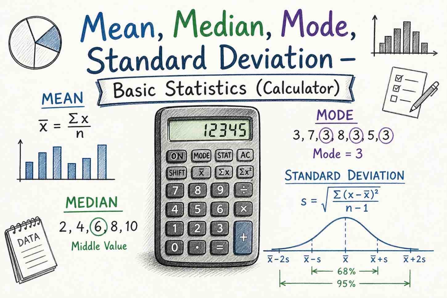
What is the mean? Formula and examples
The mean is the arithmetic average. It uses every value in the dataset, which makes it useful when the data is balanced and there are no extreme outliers.
Mean formula:
\[ \text{Mean} = \bar{x} = \frac{\text{sum of all values}}{\text{number of values}} \]
Or, using symbols:
\[ \bar{x} = \frac{x_1 + x_2 + x_3 + \cdots + x_n}{n} \]
How to calculate the mean
- Add every value in the dataset.
- Count how many values there are.
- Divide the total by the count.
Example: mean of test scores
Problem: Find the mean of 78, 85, 92, 88 and 95.
Step 1: Add the values: 78 + 85 + 92 + 88 + 95 = 438.
Step 2: Count the values: 5.
Step 3: Divide: 438 ÷ 5 = 87.6.
Answer: The mean is 87.6.
Important: The mean can be pulled upward or downward by outliers. For example, one very expensive house can make the mean house price look much higher than what most buyers actually see.
What is the median? Formula and examples
The median is the middle value after the data is ordered from smallest to largest. It is often better than the mean when the data has outliers or is skewed.
Median rule:
For an odd number of values, the median is the single middle value.
For an even number of values, the median is the average of the two middle values.
How to calculate the median
- Arrange the values from smallest to largest.
- Count the values.
- If the count is odd, choose the middle value.
- If the count is even, average the two middle values.
Example: median with odd number of values
Problem: Find the median of 15, 23, 8, 42 and 31.
Step 1: Order the values: 8, 15, 23, 31, 42.
Step 2: The middle value is 23.
Answer: The median is 23.
Example: median with even number of values
Problem: Find the median of 12, 18, 22, 25, 30 and 35.
Step 1: The values are already ordered.
Step 2: The two middle values are 22 and 25.
Step 3: (22 + 25) ÷ 2 = 23.5.
Answer: The median is 23.5.
What is the mode? Definition and examples
The mode is the value that appears most often. It is especially useful when you want to know the most common score, response, size, category or repeated value.
Mode rule: Mode = the value or values with the highest frequency.
A dataset can have one mode, two modes, more than two modes, or no mode.
How to find the mode
- List the values.
- Count how many times each value appears.
- Choose the value or values that appear most often.
Example: one mode
Problem: Find the mode of 5, 7, 5, 9, 5, 12, 7 and 5.
5 appears 4 times, 7 appears 2 times, and the other values appear once.
Answer: The mode is 5.
Example: two modes
Problem: Find the mode of 10, 15, 10, 20, 15, 25, 10 and 15.
10 appears 3 times and 15 appears 3 times. Both are tied for highest frequency.
Answer: The dataset is bimodal, with modes 10 and 15.
What is the range? Formula and examples
The range measures the spread of a dataset. It is the difference between the largest and smallest values. A larger range means the data is more spread out; a smaller range means the values are closer together.
Range formula:
\[ \text{Range} = \text{Maximum value} - \text{Minimum value} \]
Example: calculating range
Problem: Find the range of 18°C, 22°C, 15°C, 25°C, 20°C, 17°C and 23°C.
Maximum: 25°C.
Minimum: 15°C.
Calculation: 25 − 15 = 10°C.
Answer: The range is 10°C.
Range is quick, but it only uses two values. If one value is an outlier, the range can look much larger than the spread of most values. For deeper spread analysis, use standard deviation or interquartile range.
Comparing mean, median, mode and range
Use this table to choose the right measure for the question in front of you.
| Measure | Type | Best used for | Affected by outliers? |
|---|---|---|---|
| Mean | Central tendency | Balanced numerical data where every value matters | Yes |
| Median | Central tendency | Skewed data, income, house prices or data with outliers | No |
| Mode | Central tendency | Most common values, categories or repeated scores | No |
| Range | Spread | Quick view of variability | Yes |
Real-world applications
Education
Teachers use the mean to calculate class averages, the median to understand typical performance, the mode to find the most common score or misconception, and the range to see how spread out scores are. For grade work, use the grade calculator.
Business and economics
Businesses use mean for average sales, median for typical salaries or house prices, mode for popular products, and range for price or performance variation.
Science and healthcare
Researchers use these measures to summarize observations, patient readings, survey responses and experimental results before moving into more advanced analysis.
Interactive calculator: mean, median, mode and range
Statistics calculator
Enter your data values separated by commas to calculate mean, median, mode and range instantly.
Use numbers only, separated by commas. Example: 12, 15, 18, 15.
Common mistakes to avoid
1. Forgetting to order data for median: Always arrange values before finding the middle.
2. Confusing mean and median: Mean is the arithmetic average; median is the middle value.
3. Reporting mode incorrectly: The mode is the value that appears most often, not the number of times it appears.
4. Ignoring units: Add units such as dollars, marks, degrees or minutes when they matter.
5. Using mean with outliers: If the data has extreme values, the median may be more representative.
6. Assuming there is always one mode: A dataset can have no mode or multiple modes.
7. Overrelying on range: Range is useful, but it only uses the maximum and minimum values.
Practice problems
Problem 1
Books read in a month: 3, 5, 7, 3, 8, 5, 12, 3, 5, 7. Find the mean, median, mode and range.
Problem 2
Daily high temperatures: 72, 68, 75, 70, 73, 69, 71. Calculate all four measures and explain the spread.
Problem 3
Test scores: 88, 92, 76, 88, 95, 88, 84, 90. Find all four measures and decide which best represents typical performance.
Solutions
Problem 1: Mean = 5.8, median = 5, mode = 3 and 5, range = 9.
Problem 2: Mean ≈ 71.1, median = 71, no mode, range = 7.
Problem 3: Mean = 87.6, median = 88, mode = 88, range = 19. The mode and median both represent typical performance well here.
Related RevisionTown statistics resources
Use these internal resources when you need a calculator, a deeper statistics lesson, or the next topic after mean, median, mode and range.
- Statistics Calculator for broader descriptive statistics calculations.
- Mean Median Mode Calculator for quick answer checks.
- Standard Deviation Calculator for a stronger measure of spread than range.
- Statistics Formulas for formula review.
- Single Variable Statistics for school-level statistics practice.
- SAT Mathematics for exam-style math review.
Frequently asked questions
The mean is the arithmetic average. The median is the middle value after ordering the data. The mean uses all values but is affected by outliers; the median is usually better when data is skewed.
Count how often each value appears. The value that appears most often is the mode. If two values tie, the dataset is bimodal. If all values appear equally often, there is no mode.
Range tells you how spread out the values are by subtracting the smallest value from the largest value. A bigger range means more spread.
Use the median when the dataset contains outliers or is skewed, such as income, house prices, or any data with a few unusually large or small values.
Yes. A dataset can have two modes, many modes, or no mode. Multiple modes occur when more than one value ties for the highest frequency.
Order the values, find the two middle numbers, add them together, and divide by 2.
They summarize data quickly. Mean, median and mode describe typical values, while range shows how spread out the values are.
Advanced topics: beyond the basics
Weighted mean
A weighted mean gives some values more importance than others. GPA and category-weighted grades often use weighted means. See the GPA planning guide for a related example.
Interquartile range
The interquartile range measures the spread of the middle 50% of data. It is more resistant to outliers than the full range.
Standard deviation
Standard deviation measures how far values tend to sit from the mean. It uses all values, so it gives a richer picture of spread than range.
Final takeaway
Mean, median, mode and range are the foundation of descriptive statistics. Mean gives the average, median gives the middle, mode gives the most common value, and range gives the spread. Once you can calculate all four, you can summarize most simple datasets clearly and choose the measure that best fits the situation.
For balanced numerical data, start with the mean. For skewed data or outliers, check the median. For repeated values or categories, use the mode. For a fast view of variability, calculate the range.