IB Mathematics: Analysis and Approaches Higher Level
Functions Formulae for AA HL Only
A complete higher-level guide to polynomial functions, factor and remainder theorems, roots, advanced rational functions, symmetry, restricted inverses, function inequalities, transformations and modulus problems.
Higher-level functions are not simply longer versions of SL questions. They require you to move deliberately between algebra, graphs, structure and technology. A factor theorem calculation may reveal a root; a root changes the graph; a graph may determine an inequality; a domain restriction may make an inverse possible; and a transformation can create new asymptotes or erase the sign of the original function.
The formulas in this guide are therefore presented with conditions and interpretation. You will learn what each result tells you, when it is valid, which details belong on a graph and how to build an examination solution that communicates more than calculator output.

What Functions content is AA HL only?
The official additional higher-level sequence runs from AHL 2.12 to AHL 2.16. AHL 2.12 develops polynomial functions, their graphs and equations, zeros, roots, factors, the factor and remainder theorems, and the sum and product of roots. AHL 2.13 extends rational functions to forms with quadratic numerators or denominators and requires graphs with every relevant vertical, horizontal or oblique asymptote and axis intercept.
AHL 2.14 covers odd and even functions, including periodic examples, and extends inverse work to functions that need a domain restriction. It also includes self-inverse functions. AHL 2.15 asks students to solve g(x)≥f(x) graphically and analytically. AHL 2.16 investigates the graphs of |f(x)|, f(|x|), 1/f(x), f(ax+b) and [f(x)]², plus modulus equations and inequalities.
Shared SL foundation
Function notation, domain and range, composites, basic inverses, quadratics, simple reciprocal/rational functions, exponentials, logarithms, transformations and equations.
Additional HL development
General polynomial structure, root relationships, harder rational behavior, symmetry, restricted or self-inverses, function inequalities and transformations that depend on the sign or input.
This separation prevents two common revision problems. SL students should not be overloaded with content outside their course, while HL students must not mistake familiarity with basic graphs for mastery of higher-level structure.
AA HL Functions quick formula sheet
| Idea | Formula or test | Meaning |
|---|---|---|
| Remainder theorem | Remainder when P(x) is divided by x−a is P(a) | Evaluates a linear-divisor remainder without division |
| Factor theorem | x−a is a factor ⇔ P(a)=0 | Connects factors, roots, zeros and x-intercepts |
| Sum of all roots | r1+⋯+rn=−an−1/an | For anxn+⋯+a0=0, counting multiplicity |
| Product of all roots | r1⋯rn=(−1)na0/an | Works without finding individual roots |
| Even function | f(−x)=f(x) | Symmetry in the y-axis |
| Odd function | f(−x)=−f(x) | Rotational symmetry of order two about the origin |
| Inverse verification | f(f−1(x))=x | With the appropriate domains and ranges |
| Self-inverse | f(f(x))=x | The function equals its own inverse |
| Function inequality | g(x)≥f(x) ⇔ g(x)−f(x)≥0 | Compare graphs or solve a sign problem |
| Output modulus | y=|f(x)| | Reflect negative output portions above the x-axis |
| Input modulus | y=f(|x|) | Copy the right-hand half of f into the left half |
| Reciprocal transform | y=1/f(x) | Zeros of f usually become vertical asymptotes |
| Squared output | y=[f(x)]² | Outputs are non-negative; zeros are preserved |
Polynomial functions, equations, zeros and graphs
A polynomial function has the form P(x)=anxn+an−1xn−1+⋯+a1x+a0, where an≠0. Its degree n and leading coefficient determine end behavior. Zeros are values of x for which P(x)=0; real zeros appear as x-intercepts, roots solve the equation, and each corresponding linear expression x−r is a factor.
Multiplicity changes how a graph meets the axis. At a simple root the graph normally crosses. At an even-multiplicity root it touches and turns. At an odd multiplicity greater than one it crosses with a flattened shape. The exact appearance also depends on the remaining factors, but multiplicity supplies essential local information.
Worked example: build a polynomial from roots
A monic quartic has roots 2, −1 and 3, with −1 repeated. Then P(x)=(x−2)(x+1)²(x−3). The graph crosses at 2 and 3, touches at −1, and has positive end behavior on both sides because it is a monic even-degree polynomial. Expanding is unnecessary unless coefficients are required.
A degree-n polynomial has exactly n complex roots when multiplicity is counted. Non-real roots of a polynomial with real coefficients occur in conjugate pairs. This connects Functions to the AA HL complex-number work in Number and Algebra AA HL Only.
Factor and remainder theorems
The remainder theorem states that division of P(x) by x−a leaves remainder P(a). The factor theorem is the zero-remainder case: x−a is a factor if and only if P(a)=0. Be careful with divisors such as 2x+3. Rewrite the corresponding zero as x=−3/2 and evaluate P(−3/2).
x−a is a factor ⇔ P(a)=0
Worked example: find an unknown coefficient
Let P(x)=x³+kx²−5x+6, and suppose x−2 is a factor. Then P(2)=8+4k−10+6=4+4k=0, so k=−1. The theorem converts the factor statement directly into a linear equation.
Worked example: specified remainder
If dividing Q(x)=2x³−3x²+mx+4 by x+1 leaves remainder 7, then Q(−1)=7. Thus −2−3−m+4=7, giving −1−m=7 and m=−8. Substituting x=1 would correspond to divisor x−1, not x+1.
Sum and product of polynomial roots
For anxn+an−1xn−1+⋯+a0=0 with roots r1,…,rn, the official higher-level relationships are:
Πri = (−1)na0/an
Roots are counted with multiplicity and may be complex. The alternating sign in the product comes from expanding an(x−r1)⋯(x−rn). For a cubic ax³+bx²+cx+d, the sum is −b/a and the product is −d/a. For a quartic, the product is +e/a.
Worked example: find a missing root without solving
The polynomial 2x³−5x²−4x+3 has roots α, β and γ. Their sum is 5/2 and their product is −3/2. If α+β=1, then γ=5/2−1=3/2. The product then gives αβ=(−3/2)/(3/2)=−1. This obtains symmetric information without the individual values of α and β.
When a problem asks for a sum such as α²+β²+γ², rewrite it using symmetric expressions: (α+β+γ)²−2(αβ+αγ+βγ). For a cubic, the pairwise sum is c/a. Although the official headline emphasizes sum and product, coefficient comparison gives a powerful systematic method.
Polynomial division and structural rewriting
Polynomial long division expresses a numerator as divisor × quotient + remainder. It is useful for factorization after discovering a root and for finding an oblique asymptote of a rational function. Synthetic division is a compact alternative for a divisor x−a, but long division remains reliable for general divisors.
Worked example: divide by a linear factor
Divide x³−2x²−5x+6 by x−1. Synthetic division with coefficients 1, −2, −5, 6 gives quotient x²−x−6 and remainder 0. Hence P(x)=(x−1)(x²−x−6)=(x−1)(x−3)(x+2).
Include missing powers with zero coefficients. Dividing x³+4x−1 requires the coefficient list 1, 0, 4, −1. Omitting the zero shifts every later coefficient and corrupts the quotient.
Advanced rational functions
The additional HL course includes rational functions such as a linear numerator over a quadratic denominator and a quadratic numerator over a linear denominator. A complete analysis combines algebraic domain restrictions, intercepts, sign, asymptotes and graphical behavior.
Begin by factorizing numerator and denominator where possible. Record denominator zeros as excluded domain values before cancelling anything. If a common factor cancels, the simplified expression may have a removable hole at the excluded value rather than a vertical asymptote. Non-cancelled denominator zeros usually produce vertical asymptotes.
Worked example: analyze a rational function
Consider f(x)=(x²+1)/(x−2). The domain excludes 2. Long division gives f(x)=x+2+5/(x−2), so the vertical asymptote is x=2 and the oblique asymptote is y=x+2. There are no real x-intercepts because x²+1≠0 for real x. The y-intercept is f(0)=−1/2.
Vertical, horizontal and oblique asymptotes
| Feature | How to find it | Check |
|---|---|---|
| Vertical asymptote | Non-cancelled denominator zero x=a | Examine one-sided behavior; a cancelled factor may be a hole |
| Horizontal asymptote | If numerator degree is lower: y=0; if equal: ratio of leading coefficients | A graph may cross a horizontal asymptote |
| Oblique asymptote | When numerator degree is one greater, use polynomial division | The quotient line is approached as |x| grows |
| x-intercept | Numerator zero that remains in the domain | Do not include a cancelled excluded value |
| y-intercept | f(0), when 0 belongs to the domain | State as coordinate (0,f(0)) |
Asymptotes describe limiting behavior, not walls in every direction. A rational graph cannot cross a vertical asymptote because the function is undefined there, but it can cross a horizontal or oblique asymptote at a finite input. Use sign checks or technology to place branches accurately.
Worked example: horizontal asymptote
For g(x)=(3x²−2)/(2x²+5x−3), numerator and denominator have equal degree, so the horizontal asymptote is y=3/2. Factor the denominator to locate possible vertical asymptotes, then check whether the numerator shares either factor before finalizing the graph.
Odd, even and periodic functions
An even function satisfies f(−x)=f(x) and has y-axis symmetry. An odd function satisfies f(−x)=−f(x) and has origin symmetry. The domain must also be symmetric about zero for the classification to make sense across all required inputs.
Worked example: algebraic symmetry test
Let f(x)=x⁵−3x³+2x. Then f(−x)=−x⁵+3x³−2x=−f(x), so f is odd. By contrast, x⁴+2x²−7 is even. A mixture such as x³+x² is generally neither.
Periodicity and parity can coexist. Cosine is even and periodic; sine is odd and periodic. Do not infer parity from one attractive section of a graph. Apply the definition or verify the full symmetry over the domain.
Restricted inverses and self-inverse functions
A function needs to be one-to-one on its domain before its inverse is a function. A quadratic on all real numbers fails the horizontal-line test, but a restriction such as x≥h or x≤h selects one branch. The inverse’s domain is the original range, and its range is the original domain.
To find an inverse algebraically, write y=f(x), solve for x in terms of y, interchange the variable labels, and state the new domain. The graphs of f and f−1 reflect in y=x.
Worked example: restrict before inverting
Let f(x)=(x−2)²+1 with domain x≥2. Then y−1=(x−2)² and the domain selects the positive square root: x=2+√(y−1). Therefore f−1(x)=2+√(x−1) with domain x≥1. Choosing the negative root would correspond to the other branch.
A self-inverse function satisfies f−1=f, equivalently f(f(x))=x on the appropriate domain. Its graph is symmetric in y=x. The reciprocal function f(x)=1/x on nonzero real numbers is a standard example.
Solving g(x) ≥ f(x)
Graphically, solve by finding where the graph of g lies on or above the graph of f. Intersections form candidate boundaries. Analytically, move everything to one side and solve h(x)=g(x)−f(x)≥0 using factorization, roots and a sign chart.
Worked example: cubic comparison
Solve x³−4x≥x²−4. Rearranging gives x³−x²−4x+4≥0. Factor by grouping: (x−1)(x²−4)=(x−1)(x−2)(x+2)≥0. A sign chart across −2, 1 and 2 gives the solution [−2,1]∪[2,∞). Equality includes the boundary roots.
For rational comparisons, include domain restrictions and use a sign chart with both numerator and denominator critical values. Never multiply an inequality by an expression of unknown sign without splitting cases, because the inequality direction may reverse.
Advanced graph transformations
Output modulus: y=|f(x)|
Keep the portions of f on or above the x-axis. Reflect every negative-output portion upward. The zeros stay fixed, the range becomes non-negative, and sharp corners can appear where a crossing is reflected.
Input modulus: y=f(|x|)
For x≥0 the graph is unchanged. Reflect that right-hand part into the left half-plane. The original negative-input portion is discarded. The transformed graph is even wherever it is defined.
Reciprocal output: y=1/f(x)
Zeros of f become excluded inputs and typically vertical asymptotes of 1/f. Inputs where f=1 or −1 are fixed at the same output. Large magnitudes of f become values close to zero; values of f close to zero produce large reciprocal magnitudes. The reciprocal keeps the sign of f.
Linear input: y=f(ax+b)
Solve ax+b=u to track important original inputs u. The graph has horizontal scale factor 1/|a|, with a reflection in the y-axis when a<0, and the input expression places the horizontal shift at −b/a. Working from the bracket’s zero avoids memorising the shift with the wrong sign.
Squared output: y=[f(x)]²
All outputs become non-negative. Zeros remain zeros, outputs 1 and −1 both become 1, and sign information is lost. This is not the same as f(x²), which changes the input rather than the output.
Worked example: transform a quadratic
Take f(x)=x²−4. For |f(x)|, the section between −2 and 2 lies below the x-axis and reflects upward, creating three upward arcs joined at the zeros. For f(|x|), nothing changes because the original quadratic is already even. For 1/f(x), x=±2 become vertical asymptotes and y=0 is a horizontal asymptote.
Modulus equations and inequalities
For a simple expression, |u|=k with k≥0 means u=k or u=−k. The inequality |u|≤k means −k≤u≤k, while |u|≥k means u≤−k or u≥k. When u is a complex function rather than a linear expression, graphing and sign analysis may be clearer.
Worked example: quadratic inside a modulus
Solve |x²−5x+4|≤2. This is equivalent to −2≤x²−5x+4≤2. Solve both inequalities: x²−5x+2≤0 and x²−5x+6≥0. The first holds between (5−√17)/2 and (5+√17)/2; the second holds outside [2,3]. Intersect the sets carefully rather than treating the two inequalities as alternatives.
For an equation or inequality involving functions such as |3x arccos x|>1, respect the domain before using technology. Graph the relevant sides on the valid domain, find boundary intersections to appropriate accuracy, test intervals and report endpoints with correct inclusion.
Technology: use it to investigate, not replace reasoning
The official guide explicitly allows technology where an analytic approach is not appropriate. A graphing calculator or dynamic graphing package is especially useful for higher-degree roots, rational branches, intersections and transformed graphs. Before trusting the display, enter brackets correctly, choose a window based on algebraic features and verify that apparent asymptotes are not merely steep curves.
Use algebra to predict what technology should show: degree and leading coefficient for end behavior, denominator zeros for exclusions, quotient for an oblique asymptote, parity for symmetry and roots for interval boundaries. Then use the graph to refine, confirm or reveal behavior. Record the equation and interval in the written solution; unexplained screenshots or decimal lists are not enough.
How to connect an equation, graph and solution set
Higher-level functions questions often look like separate algebra and graphing tasks, but they usually test one connected idea. An equation tells you where two expressions have the same output. A graph displays those equal outputs as intersections. An inequality asks on which intervals one output is above or below the other. Moving deliberately between these three representations makes unfamiliar problems much easier to organize.
Begin with the algebraic structure rather than entering the complete expression into a calculator immediately. For a polynomial, identify its degree, leading term and any obvious factors. For a rational function, factor the numerator and denominator before cancelling anything, and keep every excluded input in view. For a transformed function, decide whether the instruction changes the input, the output or both. This first pass predicts the important x-values and prevents a misleading calculator window from controlling the solution.
A feature-map method for rational functions
Suppose r(x)=(x²−1)/(x−1). Factoring gives (x−1)(x+1)/(x−1), but the original domain still excludes x=1. The simplified rule is y=x+1 for x≠1, so the graph is a line with a hole at (1,2), not a line with a vertical asymptote. This small example captures an essential habit: simplification changes the visible formula but does not restore a value excluded by the original expression.
Now compare s(x)=(x²+1)/(x−1). No factor cancels. Division gives s(x)=x+1+2/(x−1). The denominator creates the vertical asymptote x=1, while the quotient gives the oblique asymptote y=x+1. Because the numerator has no real zero, neither branch crosses the x-axis. A calculator becomes a confirmation tool once these features are known.
Build a sign chart from boundaries, not guesses
For an inequality such as (x−3)/(x+2)≥0, the boundaries are the zero x=3 and the exclusion x=−2. These split the real line into three intervals. Test one value in each interval, include 3 because equality is allowed, and exclude −2 because the function is undefined. The result is x∈(−∞,−2)∪[3,∞). Multiplying both sides by x+2 without controlling its sign could reverse the inequality on part of the domain, which is why the sign-chart method is safer.
Read transformation chains in the correct order
For y=|f(2x−4)|, first rewrite the input as 2(x−2). The input transformation compresses the graph horizontally by factor 1/2 and shifts its key inputs two units right. The outside modulus then reflects every negative output above the x-axis. A point (u,v) on the original graph maps to ((u+4)/2, |v|). Writing this point mapping is a reliable check when a verbal transformation description feels ambiguous.
The same connection supports an exam-quality conclusion. State the exact boundaries when possible, show which points are excluded, give the requested interval or coordinate accuracy and finish with a sentence that answers the question. Correct working that stops at a calculator display or an unsolved equation may not communicate the solution set clearly enough.
AA HL Functions exam workflow
- State the domain. Record denominator restrictions, square-root restrictions and any imposed inverse branch.
- Choose a useful form. Factor for roots and signs; divide for asymptotes; complete a square for restriction and inverse work.
- Connect algebra and graph. Mark intercepts, multiplicities, symmetry, asymptotes and end behavior.
- Preserve exact values. Use coefficient relationships before approximating roots.
- Solve boundaries first. For inequalities, find every root, intersection, exclusion or modulus change point.
- Test intervals. Do not infer signs from an unreliable not-to-scale sketch.
- Verify transformations. Decide whether the change acts on input or output.
- Use technology transparently. State the functions, window/domain logic and required accuracy.
Common mistakes and how to repair them
| Mistake | Why it fails | Repair |
|---|---|---|
| Using P(a) for divisor x+a | The divisor zero is −a | Set the divisor equal to zero before substituting |
| Ignoring repeated roots | Sum/product formulas count multiplicity | List roots with repetition before applying relationships |
| Calling every denominator zero an asymptote | A common factor may create a removable hole | Factor and preserve domain restrictions before cancellation |
| Forgetting an oblique asymptote | Degree difference one requires division | Divide numerator by denominator and use the quotient |
| Finding an inverse without restriction | A many-to-one function does not have a functional inverse | Choose and state a one-to-one domain branch |
| Confusing |f(x)| with f(|x|) | One changes outputs; the other changes inputs | Describe the transformation in words before sketching |
| Multiplying a rational inequality by its denominator | The denominator’s sign may reverse the inequality | Use a combined sign chart with exclusions |
| Reporting graph intersections only | It omits the intervals where one graph is above the other | Test each region and use interval notation |
| Trusting a default calculator window | It may hide roots, branches or asymptotes | Predict features algebraically and select a justified window |
Mixed higher-level worked problems
Problem 1: roots and a parameter
The cubic x³−4x²+kx+6 has roots α, β and γ, and one root is −1. The factor theorem gives −1−4−k+6=0, so k=1. The sum of roots is 4; therefore the other two roots sum to 5. Their total product is −6, so their product is 6. Hence they solve t²−5t+6=0 and are 2 and 3.
Problem 2: rational graph from division
For f(x)=(2x²−3x+4)/(x−1), division gives 2x−1+3/(x−1). Thus x=1 is a vertical asymptote and y=2x−1 is oblique. The y-intercept is −4. The quadratic numerator has discriminant 9−32<0, so there are no real x-intercepts. These facts determine the essential branch placement before technology is used.
Problem 3: inequality involving two functions
Let f(x)=x² and g(x)=3x+4. Solve g(x)≥f(x): 3x+4≥x², so x²−3x−4≤0. Factor to (x−4)(x+1)≤0. The upward quadratic is non-positive between its roots, giving −1≤x≤4. Graphically, the line lies above the parabola between the intersections.
Fourteen-day AA HL Functions revision plan
| Day | Focus | Evidence of mastery |
|---|---|---|
| 1 | Shared SL function prerequisites | Domain, range, composites, inverses and transformations are fluent |
| 2 | Polynomial graphs and multiplicity | End behavior and axis behavior predicted from factors |
| 3 | Factor and remainder theorems | Divisor sign and parameter equations handled accurately |
| 4 | Sum and product of roots | Multiplicity and alternating product sign correct |
| 5 | Polynomial division | Missing powers included and quotient verified |
| 6 | Rational domains and intercepts | Holes distinguished from vertical asymptotes |
| 7 | Horizontal and oblique asymptotes | Degree comparison and division used without graph guessing |
| 8 | Odd, even and periodic functions | Algebraic definition and full-domain symmetry both checked |
| 9 | Restricted inverses | Original domain and inverse domain/range stated |
| 10 | Self-inverse functions | Composition verifies f(f(x))=x |
| 11 | Polynomial and rational inequalities | Complete sign charts with included/excluded boundaries |
| 12 | |f|, f(|x|) and [f]² | Input and output transformations never confused |
| 13 | 1/f and f(ax+b) | Zeros, asymptotes, horizontal scale and shift tracked |
| 14 | Mixed exam set and error log | Methods selected independently and repeated errors repaired |
Start each session with retrieval from two earlier days. Complete one algebraic question, one graph interpretation and one technology-supported problem. Mark errors by category—domain, factor, root relationship, asymptote, symmetry, inverse, inequality, transformation or communication—and reattempt them from a blank page after a delay.
These ideas feed directly into AA HL calculus. Rational rewriting, inverse functions, transformations and graph behavior matter when differentiating, finding limits, solving optimization problems and interpreting integrals. Continue to Calculus Formulae AA HL Only after the Functions foundation is secure.
Final mastery checklist
- I connect a polynomial’s factors, roots, multiplicities, intercepts and graph behavior.
- I apply factor and remainder theorems with the correct divisor zero.
- I use sum and product relationships with repeated and complex roots counted.
- I divide polynomials and verify quotient plus remainder.
- I identify every rational-function domain restriction, intercept and asymptote.
- I distinguish holes from vertical asymptotes after cancellation.
- I prove odd or even behavior algebraically and interpret the symmetry.
- I restrict a function before finding an inverse and state domains and ranges.
- I verify a self-inverse function by composition.
- I solve function inequalities with boundaries, sign charts and correct interval notation.
- I distinguish transformations of input from transformations of output.
- I solve modulus problems while preserving domain restrictions.
- I use technology to confirm algebraic structure rather than replace it.
Frequently asked questions
Which Functions sections are AA HL only?
The additional higher-level sequence is AHL 2.12–2.16: polynomials and roots, advanced rational functions, odd/even and restricted inverses, function inequalities, advanced transformations and modulus equations or inequalities.
Does AA HL also include all SL Functions content?
Yes. HL students study the shared SL sequence before the additional material. This page assumes those foundations.
What is the difference between a root, zero and factor?
If P(a)=0, then a is a root or zero of the equation/function, the graph has a real x-intercept at a, and x−a is a factor.
Do sum and product formulas include complex roots?
Yes. Count all roots over the complex numbers with multiplicity. Non-real roots of real-coefficient polynomials occur in conjugate pairs.
Can a graph cross a horizontal or oblique asymptote?
Yes. Those asymptotes describe end behavior and can be crossed at finite inputs. A vertical asymptote is different because its input is excluded.
Does every denominator zero create a vertical asymptote?
No. A common cancelled factor can produce a removable hole. Preserve the original domain restriction and inspect the simplified form.
Why must some functions have a restricted domain before inversion?
An inverse is a function only if the original function is one-to-one. Restricting to one monotonic branch can make that possible.
What makes a function self-inverse?
A self-inverse function equals its own inverse. Verify that f(f(x))=x with compatible domains.
What is the difference between |f(x)| and f(|x|)?
|f(x)| changes negative outputs into positive outputs. f(|x|) replaces negative inputs with their positive counterparts, copying the right half of the original graph to the left.
Should I solve function inequalities graphically or analytically?
Use the method requested. For simple polynomials up to degree three, be ready for both. Technology is appropriate for more complicated functions, but explain intersections and intervals.
Is polynomial long division directly useful in Functions questions?
Yes. It factorizes after a known root and reveals the quotient or oblique asymptote of a rational function.
Will the first-assessment-2029 course change this page?
The IB has announced a revised course for first assessment in May 2029. Students in that session or later should compare this guide with the new subject guide and formula booklet supplied by their school.
Official sources and related RevisionTown guides
This guide was checked against the official IB Mathematics: Analysis and Approaches guide, the IB Diploma mathematics overview and the official Mathematics AA update page.
Continue with Functions Formulae AA SL and HL, Number and Algebra Formulae AA HL Only, Geometry and Trigonometry Formulae AA HL Only, or Calculus Formulae AA HL Only.
Editorial note: independently written educational guide. Always use your school’s official IB documents for your examination session. Last reviewed: 20 August 2026.