
Probability Between Two Z-Scores Calculator
A probability between two z-scores calculator determines the area under the standard normal curve between two z-values, representing the probability or proportion of data falling within that range, computed by finding the cumulative probability for each z-score and subtracting to find the area between them using the standard normal distribution table or cumulative distribution function. This essential statistical tool calculates probabilities for any interval on the normal distribution, converts percentages to z-scores, determines confidence intervals, identifies probability ranges, and provides visual representations of areas under the curve essential for students, researchers, statisticians, quality control professionals, and anyone conducting hypothesis testing, confidence interval estimation, process capability analysis, or understanding probability distributions in statistics, research methodology, quality management, psychometrics, and data science applications requiring normal distribution probability calculations.
📊 Probability Between Z-Scores Calculator
Calculate area under normal curve between z-scores
Probability Between Two Z-Scores
Find area under curve between z₁ and z₂
Probability Above Z-Score
Find area in right tail (P(Z > z))
Probability Below Z-Score
Find area in left tail (P(Z < z))
Understanding Probability Between Z-Scores
The probability between two z-scores represents the area under the standard normal curve between those values. This area corresponds to the proportion of data or probability that falls within that range. For example, the probability between z = -1 and z = +1 is approximately 0.6827 or 68.27%, meaning about 68% of data in a normal distribution falls within one standard deviation of the mean.
Formula for Probability Between Z-Scores
General Formula
Probability Between Two Z-Scores:
\[ P(z_1 < Z < z_2) = P(Z < z_2) - P(Z < z_1) \]
\[ P(z_1 < Z < z_2) = \Phi(z_2) - \Phi(z_1) \]
Where:
\( \Phi(z) \) = cumulative distribution function
\( P(Z < z) \) = area to the left of z
\( z_1 \) = lower z-score
\( z_2 \) = upper z-score
Related Formulas
Probability Above Z-Score:
\[ P(Z > z) = 1 - P(Z < z) = 1 - \Phi(z) \]
Probability Below Z-Score:
\[ P(Z < z) = \Phi(z) \]
Step-by-Step Calculation
Example 1: Probability Between z = -1 and z = +1
Problem: Find P(-1 < Z < 1)
Step 1: Find P(Z < 1)
From z-table: P(Z < 1.00) = 0.8413
Step 2: Find P(Z < -1)
From z-table: P(Z < -1.00) = 0.1587
Step 3: Subtract probabilities
P(-1 < Z < 1) = P(Z < 1) - P(Z < -1)
= 0.8413 - 0.1587
= 0.6826
Answer: 0.6826 or 68.26%
Interpretation: About 68% of data falls within 1 standard deviation of the mean (empirical rule).
Example 2: 95% Confidence Interval
Problem: Find P(-1.96 < Z < 1.96)
Calculation:
P(Z < 1.96) = 0.9750
P(Z < -1.96) = 0.0250
P(-1.96 < Z < 1.96) = 0.9750 - 0.0250 = 0.95
Answer: 0.95 or 95%
Application: This is the basis for 95% confidence intervals in statistics.
Common Z-Score Probabilities
| Z-Score Range | Probability | Percentage | Application |
|---|---|---|---|
| -1.00 to +1.00 | 0.6827 | 68.27% | 68% empirical rule (±1 SD) |
| -1.645 to +1.645 | 0.9000 | 90.00% | 90% confidence interval |
| -1.96 to +1.96 | 0.9500 | 95.00% | 95% confidence interval |
| -2.00 to +2.00 | 0.9545 | 95.45% | 95% empirical rule (±2 SD) |
| -2.576 to +2.576 | 0.9900 | 99.00% | 99% confidence interval |
| -3.00 to +3.00 | 0.9973 | 99.73% | 99.7% empirical rule (±3 SD) |
Z-Table Reference (Selected Values)
| Z-Score | P(Z < z) | P(Z > z) | Percentile |
|---|---|---|---|
| -3.00 | 0.0013 | 0.9987 | 0.13% |
| -2.00 | 0.0228 | 0.9772 | 2.28% |
| -1.00 | 0.1587 | 0.8413 | 15.87% |
| 0.00 | 0.5000 | 0.5000 | 50.00% |
| +1.00 | 0.8413 | 0.1587 | 84.13% |
| +2.00 | 0.9772 | 0.0228 | 97.72% |
| +3.00 | 0.9987 | 0.0013 | 99.87% |
Real-World Applications
Quality Control
- Process capability: Percentage of products within specification limits
- Six Sigma: Calculate defect rates (z = ±6 means 3.4 defects per million)
- Control charts: Probability of measurements within control limits
- Acceptance sampling: Probability of accepting/rejecting batches
Research & Statistics
- Confidence intervals: 95% CI uses z = ±1.96
- Hypothesis testing: Critical regions for rejection
- Sample size calculation: Determine required sample sizes
- Power analysis: Calculate statistical power
Business & Finance
- Risk assessment: Probability of returns within range
- Value at Risk (VaR): Potential losses with given probability
- Portfolio analysis: Expected performance ranges
- Forecasting: Prediction intervals
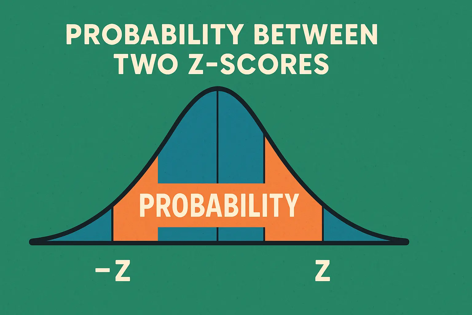
Visual Interpretation
Understanding Areas Under the Curve
Between two z-scores: Shaded area between z₁ and z₂
Formula: Area = Φ(z₂) - Φ(z₁)
Example visualizations:
- Central area: P(-1.96 < Z < 1.96) = 95% (middle area)
- Right tail: P(Z > 1.645) = 5% (right shaded area)
- Left tail: P(Z < -1.645) = 5% (left shaded area)
- Two tails: P(|Z| > 1.96) = 5% (both ends combined)
Tips for Calculating Probabilities
Best Practices:
- Always subtract correctly: P(between) = P(upper) - P(lower)
- Check z-table carefully: Verify if table shows left tail or right tail
- Use symmetry: P(Z < -a) = P(Z > a) for standard normal
- Verify with empirical rule: ±1 SD ≈ 68%, ±2 SD ≈ 95%, ±3 SD ≈ 99.7%
- Convert to percentages: Multiply probability by 100 for percentage
- Check bounds: Probability must be between 0 and 1
- Use technology: Statistical software for precise calculations
Common Mistakes to Avoid
⚠️ Calculation Errors
- Wrong subtraction order: Always subtract smaller from larger cumulative probability
- Forgetting to subtract: Must subtract P(Z < z₁) from P(Z < z₂)
- Using wrong tail: Check if z-table shows left tail, right tail, or two-tailed
- Negative probabilities: If result negative, you subtracted incorrectly
- Probability > 1: Impossible—check calculations
- Assuming normality: Standard normal calculations only valid for normal distributions
- Misreading z-table: Double-check row and column values
Frequently Asked Questions
How do you find probability between two z-scores?
Find cumulative probability for each z-score using z-table or calculator, then subtract smaller from larger. Formula: P(z₁ < Z < z₂) = P(Z < z₂) - P(Z < z₁). Example: P(-1 < Z < 1). Look up P(Z < 1) = 0.8413 and P(Z < -1) = 0.1587. Subtract: 0.8413 - 0.1587 = 0.6826 or 68.26%. This represents area under standard normal curve between the two z-values. Always use cumulative (left tail) probabilities for subtraction.
What does probability between z-scores represent?
Represents proportion or percentage of data falling within that z-score range in a normal distribution. Also equals area under standard normal curve between those z-values. Example: P(-2 < Z < 2) = 0.9545 means 95.45% of normally distributed data falls within 2 standard deviations of mean. Used for confidence intervals, hypothesis testing, quality control specifications, and understanding data distribution. Probability = area = proportion = percentage (when multiplied by 100).
How do you calculate probability above or below a z-score?
Above z-score: P(Z > z) = 1 - P(Z < z). Example: P(Z > 1.5) = 1 - 0.9332 = 0.0668 or 6.68%. Below z-score: P(Z < z) = look up directly in z-table. Example: P(Z < 1.5) = 0.9332 or 93.32%. Z-tables typically show cumulative left-tail probability. For right tail, subtract from 1. For symmetric distribution, P(Z < -a) = P(Z > a). Always verify which tail your table provides.
What is the 95% confidence interval in terms of z-scores?
95% confidence interval corresponds to z-scores of -1.96 to +1.96. P(-1.96 < Z < 1.96) = 0.95 or 95%. This means 95% of data falls within 1.96 standard deviations of mean. Leaves 5% in tails (2.5% in each tail). Used extensively in hypothesis testing and confidence interval construction. Other common intervals: 90% uses ±1.645, 99% uses ±2.576. Critical values depend on desired confidence level. Formula: CI = mean ± (z × SE).
How does the empirical rule relate to z-scores?
Empirical rule (68-95-99.7 rule) describes percentages within standard deviations: ±1 SD (z = ±1) contains 68.27% of data. ±2 SD (z = ±2) contains 95.45% of data. ±3 SD (z = ±3) contains 99.73% of data. These correspond to probabilities: P(-1 < Z < 1) ≈ 0.68, P(-2 < Z < 2) ≈ 0.95, P(-3 < Z < 3) ≈ 0.997. Provides quick estimates for normal distributions. Exact values differ slightly from common confidence intervals (e.g., 95% CI uses ±1.96, not ±2).
Can you have probability between z-scores greater than 1?
No! Probability must be between 0 and 1 (0% to 100%). If calculation gives probability > 1, error occurred—check subtraction order, z-table values, or arithmetic. Common mistake: adding instead of subtracting cumulative probabilities. Correct formula: P(z₁ < Z < z₂) = P(Z < z₂) - P(Z < z₁), not addition. Probability = 1 only if range includes entire distribution (e.g., -∞ to +∞). For any finite z-score range, probability < 1. Always verify result makes logical sense before reporting.
Key Takeaways
Understanding how to calculate probabilities between z-scores is fundamental for statistical analysis, hypothesis testing, confidence intervals, and quality control. This skill enables interpretation of normal distribution data and application of inferential statistics in research and business decision-making.
Essential principles to remember:
- Probability between z-scores = P(Z < z₂) - P(Z < z₁)
- Use cumulative (left tail) probabilities for calculations
- Always subtract smaller probability from larger
- Common ranges: ±1.96 (95%), ±1.645 (90%), ±2.576 (99%)
- Empirical rule: ±1 SD ≈ 68%, ±2 SD ≈ 95%, ±3 SD ≈ 99.7%
- Probability must be between 0 and 1
- Area under curve = probability = proportion
- Use z-table or calculator for precise values
- Verify calculations with known benchmarks
- Apply to confidence intervals and hypothesis tests
Getting Started: Use the interactive calculator at the top of this page to find probabilities between any two z-scores, above a z-score, or below a z-score. Enter your z-values and receive instant results with visual representations, step-by-step calculations, and interpretations. Perfect for students, researchers, quality control professionals, and anyone working with normal distributions and statistical analysis.