
IB Mathematics: Applications and Interpretation
Functions Formulae for AI SL and HL
A complete guide to straight lines, function notation, graph features, modelling, exponential and sinusoidal behaviour, plus AI HL composite functions, inverses, transformations and logarithmic linearisation.
Reviewed against the current IB Mathematics: Applications and Interpretation guide. Topic 2 is compulsory at both levels; additional higher-level content is identified clearly below.
Functions are the language of mathematical modelling. A formula links variables; a graph reveals shape and change; a table supplies evidence; and technology lets us compare a model with data. In AI, the important question is not only “can you calculate this value?” but also “what does this value mean, where is the model valid, and how well does it represent the situation?”
The official course allocates substantial teaching time to functions—31 suggested hours at SL and 42 at HL. Standard Level builds the foundations: lines, function notation, graphing, key features, model families and the modelling cycle. Higher Level includes every SL idea and extends the topic through composite and inverse functions, transformations, further models and logarithmic scales used to linearise relationships. This page combines both levels while making the boundary visible.
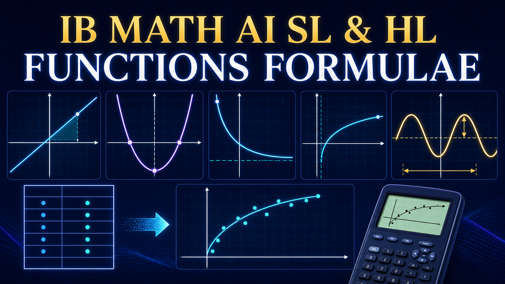
What AI SL and AI HL study in Functions
Both levels study relationships among variables and use equations, graphs and tables as complementary representations. Students investigate how parameters correspond to visible graph features and physical quantities. They choose suitable windows, fit models with technology, solve equations using intersections and evaluate whether results are sensible in context.
The central habit is translation. A constant slope in an equation should be visible as a straight graph and interpreted as a constant rate. A quadratic coefficient should predict opening direction and curvature. An exponential base or continuous rate should predict growth or decay. A sinusoidal period should correspond to a repeating time. A domain restriction should describe when inputs make mathematical and contextual sense.
| Shared AI SL and HL foundation | Additional AI HL layer |
|---|---|
| Gradient and equations of straight lines | Composite functions and identities |
| Function notation, domain, range and representations | Inverse functions and domain restrictions |
| Graphing and interpreting key features | Graph transformations and parameter effects |
| Modelling with familiar function families | Further function models and stronger algebraic connections |
| Technology-based equation solving and validation | Logarithmic scales and linearising data |
AI HL is not a separate collection that replaces SL. It builds on the shared material. An inverse-function problem still requires domain knowledge; a transformation problem still requires graph features; and logarithmic linearisation is useful only if you can interpret a straight-line gradient and intercept.
Function notation, domain, range and representations
A function assigns exactly one output to each permitted input. The notation f(x) names the output of function f when the input is x. It does not mean f multiplied by x. If f(x)=2x²−3, then f(4)=2(4)²−3=29. Parentheses protect negative or compound inputs.
f(4)=2(4)²−3=29
f(a+h)=2(a+h)²−3
The domain is the set of allowed inputs. The range is the set of resulting outputs. Restrictions may come from mathematics, data collection or context. A denominator cannot be zero; a square-root radicand must be non-negative when using real numbers; a logarithm requires a positive argument; and a time model may be limited to the observed interval.
Mathematical domain
For g(x)=1/(x−5), x=5 is excluded. For h(x)=√(x+2), real inputs require x≥−2.
Contextual domain
A population model may be defined algebraically for every real x but used only for 0≤t≤20 years because that is the reliable prediction window.
A relationship can be shown as an equation, graph, table, mapping or verbal rule. No single representation is always best. A table is concrete but finite. An equation enables calculation and manipulation. A graph displays overall structure but depends on scale and window. A well-written AI solution moves between them and explains what each contributes.
Worked example: domain from a model
A ball's height is modelled by H(t)=−4.9t²+18t+1.2. Algebraically the formula accepts all real t, but if t is time after release, use t≥0 and stop when the ball reaches the ground. The relevant domain is determined by the positive solution of H(t)=0.
The negative root may be mathematically correct yet irrelevant to the physical event. State why it is rejected.
Gradients and equations of straight lines
The gradient measures change in y per unit change in x. Given two distinct points, divide the vertical change by the horizontal change. Order must be consistent in numerator and denominator. A positive gradient rises from left to right, a negative gradient falls, zero is horizontal, and a vertical line has undefined gradient.
The slope-intercept form y=mx+c displays gradient m and y-intercept c. Point-gradient form is convenient when one point and the gradient are known. Standard form can support exact manipulation and intercept calculations.
Point-gradient: y−y₁=m(x−x₁)
Standard form: Ax+By+C=0
Worked example: equation through two points
Find the line through (2,5) and (8,17).
y−5=2(x−2)
y=2x+1
Check both points: substituting x=2 gives 5 and x=8 gives 17.
Parallel and perpendicular lines
Non-vertical parallel lines have equal gradients. Non-vertical perpendicular lines have gradients whose product is −1. Therefore the perpendicular gradient to m is −1/m when m is non-zero. Horizontal and vertical lines form a special perpendicular pair.
Perpendicular: m₁m₂=−1
In context, the gradient has units. If y is dollars and x is hours, m is dollars per hour. The intercept represents the predicted y-value when x=0, which may be meaningful, impossible or outside the data. Never interpret parameters without checking units and domain.
Direct variation and linear proportionality
Direct proportion has y=kx and passes through the origin. A line y=kx+c with c≠0 is linear but not directly proportional. The distinction matters when interpreting a fixed charge plus a usage rate.
Application: taxi model
A fare is C(d)=4.50+1.80d, where d is distance in kilometres. The gradient 1.80 means an additional 1.80 currency units per kilometre. The intercept 4.50 is the fixed starting charge. This is linear but not direct proportion.
Key graph features and what they communicate
Reading a graph means more than naming its family. Important features include intercepts, zeros, turning points, local and global maxima or minima, axis of symmetry, asymptotes, intervals of increase or decrease, domain, range and end behaviour. In an applied problem, every feature may have units and a contextual interpretation.
Intercepts and zeros
The y-intercept occurs at x=0, provided 0 belongs to the domain. An x-intercept or zero occurs where f(x)=0. Technology may give several zeros; retain only those within the relevant domain and requested interval.
x-intercepts: solve f(x)=0
For a revenue function, a zero may indicate break-even only if the model actually represents profit rather than revenue. Interpretation must match the variable definition. A point on the graph does not carry meaning independent of the model.
Turning points and axis of symmetry
A quadratic f(x)=ax²+bx+c has an axis of symmetry x=−b/(2a). The vertex lies on this line. If a>0 the vertex is a minimum; if a<0 it is a maximum. Vertex form makes the feature immediate.
Axis: x=−b/(2a)
Vertex form: f(x)=a(x−h)²+k
Vertex: (h,k)
Worked example: interpret a vertex
Profit is modelled by P(x)=−2(x−40)²+3200 for 0≤x≤80, where x is units sold in hundreds.
The vertex (40,3200) gives a maximum predicted profit of 3200 currency units when 4000 items are sold, because x=40 represents 40 hundreds. The units and scale are part of the interpretation.
Asymptotes and end behaviour
An asymptote is a line a graph approaches according to the model. Exponential decay of the form y=abx with 0<b<1 has horizontal asymptote y=0. A translated model y=abx+k has horizontal asymptote y=k. Logarithmic functions have a vertical asymptote where their argument approaches zero.
Logarithm: y=log_b(x−h)+k has vertical asymptote x=h
Approaching an asymptote does not necessarily mean reaching it. A population model approaching a carrying capacity may remain below that capacity for every finite time. A graphing window can make a curve look as though it touches an asymptote, so combine visual evidence with the formula.
Increasing and decreasing intervals
A function is increasing where larger inputs lead to larger outputs and decreasing where they lead to smaller outputs. Technology can trace or graph these intervals, while calculus later gives derivative-based criteria. At SL, interpret the shape and use appropriate numerical tools; at HL, connect these features to transformations, composite structure and later calculus work.
Core function families and formula reference
Model selection begins with recognizing shape. Do not choose a model merely because a calculator can fit it. Ask what mechanism the function represents and whether its features match the data.
| Family | Typical form | Signature behaviour | Common use |
|---|---|---|---|
| Linear | y=mx+c | Constant first differences and constant rate | Fixed-rate change and local approximations |
| Quadratic | y=ax²+bx+c | Parabola, one turning point, constant second differences | Projectile paths, area and optimization |
| Exponential | y=abx or y=Aekx | Constant ratio or constant percentage change | Population, finance, cooling and decay |
| Power | y=axn | Scaling relationship controlled by exponent n | Geometry, allometry and physical laws |
| Inverse variation | y=k/x | Product xy is constant; reciprocal curve | Rate, intensity and allocation models |
| Sinusoidal | y=a sin(b(x−c))+d | Repeating pattern with amplitude and period | Seasons, tides, sound and cyclic motion |
| Logarithmic | y=a+b ln x | Rapid early change followed by slower change | Scales, inverse exponential processes and linearisation |
Linear models
A linear model assumes constant absolute change. If x increases by one unit, y changes by m. Residuals should show no systematic curve if the model is appropriate. Extrapolation is risky because real systems rarely maintain a constant rate indefinitely.
Quadratic models
Quadratic models capture one bend and one turning point. Their first differences change linearly and their second differences are constant for equally spaced x-values. The coefficient a determines opening direction and width, while the vertex gives an optimum.
Discriminant: Δ=b²−4ac
When a quadratic comes from technology, record coefficients with sufficient precision. Rounding coefficients too early can shift roots or a maximum. Use the stored regression model for calculations where possible.
Exponential growth and decay
An exponential model has constant multiplicative change over equal x-steps. In y=abx, a is the initial value when x=0 and b is the growth factor per unit. If b>1 the model grows; if 0<b<1 it decays. A percentage rate r written as a decimal gives b=1+r for growth and b=1−r for decay.
Continuous model: y=Ae^(kx)
Growth: r>0 or k>0
Decay: −1<r<0 or k<0
Worked example: repeated percentage change
A quantity starts at 1200 and decreases by 8% each year.
After six years, Q(6)≈727.63. The multiplier is 0.92, not −0.08, because the remaining quantity is 92% of the previous year.
Sinusoidal models
A sinusoidal model represents smooth periodic behaviour. In y=a sin(b(x−c))+d, |a| is amplitude, d is the midline, c controls horizontal shift, and the period depends on angle measure. When x is in radians, period=2π/|b|. If degrees are used, period=360°/|b|.
Amplitude=|a|
Midline: y=d
Period=2π/|b| in radians
Cosine can model the same cycle with a different phase shift. Select the form that fits a natural starting feature. A tide model beginning at a maximum may be simpler with cosine. Technology can fit sinusoidal models, but the data should span enough cycles to estimate period reliably.
Inverse and power relationships
Direct variation y=kx keeps y/x constant. Inverse variation y=k/x keeps xy constant. A general power model y=axn may show positive or negative scaling depending on n. These distinctions can be tested with ratios, products and logarithmic plots.
The modelling cycle with functions
A model is a purposeful simplification, not a perfect copy of reality. The AI course emphasizes choosing, fitting, interpreting and evaluating functions in context. A strong response identifies variables and units, states assumptions, chooses a family, determines parameters, checks residuals or fit, makes predictions and comments on validity.
- Specify: define the question, variables, units and useful domain.
- Collect or inspect: understand how data were produced and whether they are reliable.
- Represent: plot the data before fitting a model.
- Choose: connect visible shape and mechanism to a plausible family.
- Fit: estimate parameters with algebra or technology.
- Validate: inspect residuals, error measures and contextual behaviour.
- Use: interpolate or cautiously extrapolate, keeping units and precision.
- Evaluate: state limitations, assumptions and a realistic validity interval.
Interpolation versus extrapolation
Interpolation predicts within the observed x-range; extrapolation predicts outside it. Interpolation is not automatically correct, but it usually relies less on untested assumptions. Extrapolation may produce impossible negative populations, unlimited growth or repeated cycles that do not persist. State clearly when a prediction goes beyond the data.
Residuals
A residual is observed minus predicted. Positive residuals lie above the fitted model, negative residuals below. A residual plot with random scatter around zero supports the chosen form; a curve or pattern suggests missing structure. Small residuals alone do not prove causation or guarantee reliable extrapolation.
eᵢ=yᵢ−ŷᵢ
Model comparison
Suppose sales rise quickly and then level off. A quadratic may fit the observed interval but eventually turns downward and becomes negative. A logistic-style or saturating model may better reflect a market limit. Compare residuals and long-term behaviour, not only the coefficient of determination.
Parameter interpretation
Parameters should be interpreted in units and context. In y=mx+c, m is output units per input unit. In y=abx, b is a multiplier per input step. In y=a sin(b(x−c))+d, |a| is half the peak-to-trough range, d is the average level, and period is a time or angle cycle. An unexplained coefficient is a missed modelling insight.
Graphing and solving with technology
Technology is central in AI, but correct use includes window choice, numerical precision and validation. Enter expressions with parentheses, distinguish multiplication from function notation, and define the same variable used in the question. Store regression models rather than retyping rounded coefficients.
Solving equations by intersections
To solve f(x)=g(x), graph both functions and find intersection x-values, or graph f(x)−g(x) and find zeros. Report solutions inside the required domain and interval. A graph can miss intersections if the window is too narrow or resolution is poor.
Break-even intersection
If revenue is R(x)=45x and cost is C(x)=1200+25x, solve R(x)=C(x).
20x=1200
x=60
The break-even output is 60 units. A graphing calculator should show the two lines intersect at (60,2700).
Choosing a graphing window
Use the domain and estimated output range to set the window. Include relevant intercepts, turning points and asymptotes. If a parabola appears linear, zoom out or shift the window. If an exponential looks flat, rescale axes. The displayed shape is evidence only after the frame of reference is suitable.
Composite functions — AI HL
A composite function applies one function to the output of another. The notation (f∘g)(x)=f(g(x)) means g acts first, followed by f. Order matters: f∘g is generally different from g∘f. A composite is defined only when x belongs to the domain of the inner function and its output belongs to the domain of the outer function.
(g∘f)(x)=g(f(x))
Worked example: order of composition
Let f(x)=2x+3 and g(x)=x²−1.
(g∘f)(x)=(2x+3)²−1=4x²+12x+8
The results are not equal. Always substitute the complete inner expression using parentheses.
Composite domains
Suppose f(x)=√x and g(x)=x−4. Then (f∘g)(x)=√(x−4), requiring x≥4. But (g∘f)(x)=√x−4 requires x≥0. The formula alone is incomplete without the domain.
Composites naturally represent multi-stage processes. A currency conversion may act after tax; a temperature formula may act after time is converted to hours; an area formula may use a radius that itself depends on time. Describing the stages helps determine order.
Application: two-stage price
A base price x first receives a 15% discount, d(x)=0.85x, then 5% tax, t(x)=1.05x. The final price is:
The final amount is 89.25% of the original. For purely multiplicative stages the order happens to give the same product, but that is a feature of this example, not a general composition law.
Inverse functions — AI HL
An inverse reverses the input-output process. If f(a)=b, then f−1(b)=a. The notation f−1 does not mean 1/f. A function must be one-to-one on its chosen domain to have a functional inverse. A horizontal-line test checks this graphically.
f(f^(−1)(x))=x
To find an inverse algebraically, write y=f(x), interchange x and y, solve for y, then state the correct domain and range. The graph of an inverse is the reflection of the original graph in the line y=x.
Worked example: linear inverse
Find the inverse of f(x)=3x−7.
x=3y−7
y=(x+7)/3
f^(−1)(x)=(x+7)/3
Check: f−1(f(x))=[(3x−7)+7]/3=x.
Restricting a quadratic domain
The function f(x)=x² is not one-to-one over all real numbers because x and −x produce the same output. Restricting the domain to x≥0 gives inverse f−1(x)=√x. Restricting to x≤0 gives f−1(x)=−√x. The chosen branch matters.
f^(−1)(x)=√x with domain x≥0
Domain and range swap under inversion. If f has domain D and range R, then f−1 has domain R and range D. In a contextual model, an inverse often answers the reverse question: instead of finding population at time t, find the time at which a target population is reached.
Function transformations — AI HL
Transformations produce related graphs from a base function. Outside changes affect vertical coordinates; inside changes affect horizontal inputs and often reverse the intuitive direction. Track important points, domain, range and asymptotes—not only the overall shape.
| Transformation | Effect on y=f(x) |
|---|---|
| f(x)+k | Translate vertically by k |
| f(x−h) | Translate horizontally right by h |
| af(x) | Vertical scale factor |a|; reflect in x-axis if a<0 |
| f(bx) | Horizontal scale factor 1/|b|; reflect in y-axis if b<0 |
| −f(x) | Reflect in the x-axis |
| f(−x) | Reflect in the y-axis |
Transformations may be combined. A reliable order is to understand the inside input change and then the outside output change, while using points to verify. If (u,v) lies on y=f(x), then a transformed coordinate can be derived rather than guessed.
Worked example: transform a parabola
Start with y=x² and form y=−2(x−3)²+5.
The graph shifts right 3, stretches vertically by factor 2, reflects in the x-axis and shifts up 5. Its vertex is (3,5), axis of symmetry x=3, and it opens downward.
Transforming asymptotes
For y=ex, the horizontal asymptote is y=0. In y=3e−2(x−1)+4, the asymptote becomes y=4. For y=ln x, the vertical asymptote is x=0; in y=ln(x−5)−2 it becomes x=5. Transforming key features is faster and safer than plotting arbitrary points.
Use transformations to interpret parameters in a model. A vertical shift may represent background level, a horizontal shift may represent delayed onset, and a vertical scale may represent amplitude or capacity. The parameter meaning depends on the family and context.
Further function models — AI HL
AI HL extends the modelling toolkit and expects students to compare models critically. A more flexible fit is not automatically better. Every additional parameter can improve in-sample accuracy while making interpretation harder and extrapolation less reliable.
Polynomial models
A polynomial of degree n can have at most n real zeros and at most n−1 turning points. End behaviour depends on degree parity and the sign of the leading coefficient. Polynomial regression can fit curved data over a limited interval, but high-degree polynomials may oscillate dramatically outside it.
Choose the lowest degree that captures meaningful structure. A quartic fit with a very high coefficient of determination may be less defensible than a quadratic supported by the process being modelled.
Logistic and saturating behaviour
Many growth processes begin approximately exponentially but slow as resources become limited. A logistic curve has an S-shape and approaches a carrying capacity. Parameter forms vary, so interpret the specific equation supplied or fitted.
Here L is the limiting level when parameters and domain have the usual interpretation, while k controls growth rate. The inflection region represents the fastest growth. A logistic model can be more plausible than unlimited exponential growth for populations or adoption, but only if the data show saturation.
Piecewise models
A piecewise function uses different rules on different intervals. It can model tax brackets, shipping costs, staged motion or interventions. Boundary notation must show whether endpoints are included. Check for continuity only when the context suggests a smooth transition.
The first rule handles the initial interval; the second begins at the threshold. Substituting x=10 into the applicable rule prevents ambiguity. Technology may require separate domain conditions for each piece.
Logarithmic scales and linearising data — AI HL
Logarithms compress wide ranges and turn certain nonlinear relationships into straight lines. A straight transformed plot helps identify model type and estimate parameters. Always record what was transformed and convert the line parameters back into the original model.
Exponential linearisation
For y=abx, take logarithms of y. Using natural logs gives ln y=ln a+x ln b, which is linear in x. A plot of ln y against x has gradient ln b and intercept ln a.
ln y=ln a+x ln b
Gradient=ln b and intercept=ln a
After fitting line Y=mx+c where Y=ln y, recover b=em and a=ec. If common logarithms are used instead, remain consistent and apply the correct inverse base.
Power-model linearisation
For y=axn, take logarithms of both variables. Then ln y=ln a+n ln x. A plot of ln y against ln x has gradient n and intercept ln a.
ln y=ln a+n ln x
Gradient=n and intercept=ln a
Worked interpretation
A log-log regression gives ln y=1.25 ln x+0.70.
a=e^0.70≈2.014
Model: y≈2.014x^1.25
The gradient becomes the power exponent. The intercept must be exponentiated; it is not the original coefficient itself.
When log transformations are valid
Real logarithms require positive arguments, so x and/or y must be positive according to the transformation. A log plot can change the visual weighting of errors: equal vertical distances in log space correspond to multiplicative differences in original space. Validate the recovered model using original-scale residuals and context, not only the transformed straightness.
A reliable exam and modelling workflow
- Define variables, units and the relevant domain.
- Identify the requested representation: equation, graph, table or interpretation.
- Estimate the expected sign, scale and number of solutions.
- Choose a function family using mechanism and shape.
- Enter the model carefully and store unrounded coefficients.
- Select a graph window that includes important features.
- Use intersections, zeros, regression or numerical solving as appropriate.
- Check solutions in the original equation and reject invalid values explicitly.
- Report suitable precision with units.
- Interpret the result and comment on model validity.
Common mistakes and how to correct them
| Mistake | Why it fails | Better habit |
|---|---|---|
| Treating f(x) as f multiplied by x | Function notation represents evaluation | Read f(x) as “the output of f at x” |
| Ignoring domain and range | Solutions may be undefined or contextually impossible | State mathematical and contextual restrictions early |
| Calling every straight line direct proportion | Direct proportion must pass through the origin | Distinguish y=kx from y=mx+c |
| Using a default graph window | Roots, vertices or asymptotes may be hidden | Choose the window from domain and estimated features |
| Rounding regression coefficients before prediction | Error may accumulate and shift results | Store the full model and round only the final answer |
| Assuming high fit means causation | Association does not establish mechanism | Discuss design, variables, residuals and limitations |
| Composing functions in the wrong order | The inner function acts first | Write f(g(x)) and substitute complete expressions |
| Confusing inverse with reciprocal | f−1(x) and 1/f(x) are different | Use input-output reversal and composition checks |
| Shifting f(x−h) left | Horizontal transformations act oppositely inside | Track a known point or solve x−h=old input |
| Leaving log-line parameters unconverted | Transformed intercept is often ln a, not a | Apply the inverse logarithm to recover the original model |
Seven-day functions revision plan
- Day 1: notation, domain, range and representation conversions.
- Day 2: gradients, line equations, parallel and perpendicular relationships.
- Day 3: graph features and core linear, quadratic and exponential families.
- Day 4: sinusoidal and power models, regression and residual interpretation.
- Day 5: technology solving, window choice, interpolation and extrapolation.
- Day 6 HL: composites, inverses and transformations. SL students use mixed modelling practice.
- Day 7 HL: further models and logarithmic linearisation. Everyone completes a timed mixed set and error review.
Frequently asked questions
Are functions compulsory in both AI SL and AI HL?
Yes. Topic 2 is compulsory at both levels. HL students study all shared SL content plus additional higher-level subtopics such as composites, inverses, transformations, further models and logarithmic linearisation.
What is the difference between a relation and a function?
A function assigns exactly one output to every permitted input. A relation may associate one input with several outputs. The vertical-line test checks whether a graph represents y as a function of x.
Is the domain always all real numbers?
No. Denominators, roots and logarithms create mathematical restrictions, while context creates practical limits. Always state the relevant domain rather than assuming every real input is meaningful.
How do I choose between linear and exponential models?
Linear data show approximately constant differences; exponential data show approximately constant ratios or percentages. Plot the data, inspect residuals and consider the process. Do not choose only by a fit statistic.
Does a high coefficient of determination prove the model is correct?
No. It describes fit under specific conditions but does not prove causation, correct mechanism or reliable extrapolation. Residuals, assumptions and long-term behaviour still matter.
When should I use sine instead of cosine?
Both can describe the same cycle with a phase shift. Choose the form that aligns naturally with a starting feature: cosine is often convenient at a maximum or minimum, while sine is convenient at a midline crossing.
Why are f∘g and g∘f usually different?
The first operation changes what the second receives. Unless the particular functions commute, reversing the order produces a different expression and model. Translate the real process into stages before composing.
Why does a quadratic need a restricted domain before inversion?
Over all real inputs, most quadratics fail the horizontal-line test. Restricting to one side of the vertex makes the function one-to-one and selects one inverse branch.
How do I solve two functions equal with a graphing calculator?
Graph both and find intersections, or graph their difference and find zeros. Set a suitable window, list all solutions in the required interval and substitute them back when practical.
What does a residual plot tell me?
Random scatter around zero supports the chosen form. Curvature, widening spread or clusters suggest that the model, variance or data structure needs attention. Residuals do not by themselves prove causal validity.
Why linearise data with logarithms?
A nonlinear exponential or power relationship can become a line after a suitable transformation. The gradient and intercept then estimate original model parameters, but they must be converted back correctly.
Can I use only calculator regression in an exam answer?
Technology may generate the model, but a complete response identifies the model, reports coefficients appropriately, shows the relevant calculation and interprets or evaluates the result in context.
Is this an official IB publication?
No. This is an independent RevisionTown teaching guide informed by official curriculum documents. The International Baccalaureate Organization is the authoritative source for course and assessment requirements.
Final Functions checklist
- I can move among equation, table and graph representations.
- I can state domain, range and contextual restrictions.
- I can calculate and interpret gradients and line parameters.
- I can identify intercepts, extrema, asymptotes and intervals of change.
- I can recognize linear, quadratic, exponential, power and sinusoidal behaviour.
- I can fit, validate and interpret a model using residuals and context.
- I can solve equations numerically and verify graphing windows.
- At HL, I can compose, invert and transform functions with domains.
- At HL, I can use logarithmic plots to linearise exponential and power models.
- I can communicate units, precision, assumptions and limitations.
Continue with the AI HL-only Functions guide for deeper higher-level practice, or return to the AI SL and HL prior-learning guide when a graphing problem reveals a foundational gap. Function fluency also supports the later AI Calculus formulae guide, where rates and areas are interpreted through graphs and models.
Official curriculum references
- IB Mathematics: Applications and Interpretation guide
- IB Applications and Interpretation curriculum update
- IB Diploma Programme mathematics overview
RevisionTown is independent and is not affiliated with or endorsed by the International Baccalaureate Organization. Verify requirements against the documents for your examination session.


